PFA Debris-Flow Runout Analysis

1 Introduction: debris-flow runout

This document reports on an update and recalibration of the linked landslide initiation and debris-flow runout models used for the Private Forest Accord (PFA, (Oregon Department of Forestry 2022)) steep-slopes modeling. These models were developed by Dan Miller and Kelly Burnett as described in Miller and Burnett (2007, 2008) with application of the models described in Burnett and Miller (2007). The original models were calibrated using landslide-initiation locations, debris tracks, and “debris-torrent”-impacted channels that were field surveyed for the 1996 Storm Study by the Oregon Department of Forestry (ODF) (Robison et al. 1999) and digitized to 10-meter line-trace DEM base maps. Several factors motivate a re-calibration and re-examination of these models. Recent work by the Oregon Department of Geology and Mineral Resources (Burns, Franczyk, and Calhoon 2022) now provides an inventory of landslide initiation points and debris-flow-runout tracks with a greater geographic and temporal range than available from the 1996 Storm Study; high-resolution DEMs derived from lidar are now available for much of Oregon (https://www.oregongeology.org/lidar/), and statistical methods and analysis tools have progressed considerably in the last 15 years.

The Miller-Burnett models identify the channels susceptible to direct impacts from debris flows originating upslope and delineate the source areas for those debris flows. Although the initiation and evolution of a landslide into a debris flow is a continuous process, the models examine landslide initiation and runout separately. This is because initiation and runout involve different sets of physical processes influenced by different sets of environmental factors. An empirical approach is used for both cases, in which statistical models are calibrated using observed landslide initiation sites and debris-flow tracks, but with the choice of predictor variables (also called the independent variables) based on current understanding of the physical processes involved. The models are linked in that the modeled potential for downslope impacts is a function of both initiation probability and runout probability. This document focuses on runout; a separate document describes the modeling done for landslide initiation.

Numerous studies have examined controls on debris-flow runout. Some specific to the Pacific Northwest include Benda and Cundy (1990); Hofmeister et al. (2002); Fannin and Rollerson (1993); Robison et al. (1999); May (2002); Lancaster et al. (2003); Miller and Burnett (2008); Guthrie et al. (2010); Coe (2011), and Reid et al. (2016). These and other studies consistently point to several factors that influence runout lengths:

• “channel gradient and confinement,

• abrupt changes in flow direction at channel junctions,

• the volume of mobilized material, and

• the size and number of trees encountered and the amount of large wood incorporated into the mobilized material.

Empirical models to predict runout length seek to calibrate observed runout lengths to measurements or estimates of these factors. Benda and Cundy (1990) used channel slope and tributary junction angles. Fannin and Wise (2001) use channel gradient and confinement, estimated volume, and changes in flow direction. Miller and Burnett (2008) used channel gradient and confinement, estimated volume, tributary junction angles, and stand-age brackets (as indicators of tree size and wood availability). Gurthie et al. (2010) used gradient, changes in flow direction, and presence/absence of mature timber. Reid et al. (2016) used estimated mobilized volume.

The Miller-Burnett models were developed for the Coastal Analysis and Modeling Study (CLAMS) specifically for characterizing potential debris-flow impacts to channels over the entire Oregon Coast Range. They were unique across modeling approaches in that they:

• linked both probability of initiation and probability of runout to calculate probability of downslope impacts,

• utilized digital elevation data to characterize topographic attributes point by point over potential runout paths,

• characterized susceptibility in terms of the proportion of landslide initiation sites and debris-flow track length (see Burnett and Miller 2007),

• and could be run over large regional extents at the resolution of available DEMs.

Although modeling approaches have evolved since 2008 (see the discussion), the Miller-Burnett models continue to offer unique capabilities. In particular, they provide calculations of runout probability from every DEM cell with a nonzero probability of landslide initiation. This capability provided the means for two primary analyses used for the PFA steep-slope prescriptions:

1. Delineation of nonfish-bearing channels that may be traversed by a debris-flow originating upslope and ranking these channels by the probability that a traversing debris flow will continue downstream and deliver material to a fish-bearing channel. These are the “Debris-flow traversal areas” defined in the PFA report (Oregon Department of Forestry 2022, 30).

2. Delineation of upslope source areas for debris flows that can travel to fish-bearing streams and ranking of those source areas in terms of the likely volume of material delivered. These are the “Sediment Source Areas” (Oregon Department of Forestry 2022, 31).

Tracking all potential debris-flow tracks from every potential source is a huge computational task that this model handles through use of survival analysis (Kalbfleisch and Prentice 2002). Survival analsyis is a statistical technique used extensively in medical and engineering analyses to quantify effects of environmental factors on expected lifespans and time to failure (e.g., of people or machine parts), but which had not been used previously for analysis of debris-flow runout. Miller and Burnett (2008) developed a survival-analysis approach in which the “lifespan” of a debris flow is measured in terms of runout distance, rather than time. This is a computationally efficient algorithm with which the runout probability for the many millions of potential initiation sites across a region can be calculated while accounting for environmental conditions point-by-point along each potential runout track.

Modeling tools for survival analysis have progressed since 2008. For this recalibration, we used the statistical language R (https://www.r-project.org/). Analyses with R are typically done using R Packages, which provide a set of well-vetted programming tools for specific applications. We used the survival and flexsurv packages to calibrate a survival model for debris-flow runout. Details of this analysis, including the code, follow in subsequent sections.

2 Methods

2.1 Survival Analysis

Empirical estimates of probable lifespan for individuals in a population are based on the distribution of lifespans measured for some sample from that population. Effects of factors that might influence lifespan are then evaluated by their effects on the shape of that distribution. Here, “lifespan” refers to the increment of time until some event of interest. In medical applications, this might involve the time that patients remain cancer free following different types of treatment. In engineering applications, this might involve how long until a machine part fails. In social applications, it might involve the length of time that a couple remains married as a function of income. See the introductory article by Emmert-Streib and Dehmer (2019) for other examples. A key aspect of survival analysis is the ability to incorporate “censured” data; that is, to use measured time spans for individuals in a sample for which the expected event does not occur prior to the end of the observation period.

Here we look at the “lifespan” of a debris flow, not in terms of time, but in terms of distance. We want to know the expected runout length as a function of environmental factors encountered along the runout path. We are interested in the factors listed in the introduction above: channel gradient and confinement, changes in flow direction, the volume of material mobilized, and the quantity of large woody debris incorporated.

2.1.1 Survival Curves

A survival curve gives the proportion of individuals in a population that survive beyond a given time. It varies from zero to one on the y axis and 0 to the length of the period of observation on the x axis. A survival curve for debris flows indicates the proportion of events in a population of debris flows that runout beyond a given distance. An empirical estimate of the survival curve is obtained from the cumulative distribution of measured debris-flow-track lengths. For a given sample of debris-flow runout lengths, the survival curve is estimated as the proportion of tracks in the sample longer than a given length:

\[ S(x) \approx \frac{\# \: tracks \: longer \: than \: x}{N} \tag{1}\]

where \(N\) is the total number of tracks (see Emmert-Streib and Dehmer 2019 for a concise description). The shape of this distribution is determined by the probability that any individual debris flow will stop in the next interval of travel along its travel path. This probability is called the hazard rate and is defined as

\[ h(x) = \lim\limits_{\Delta x \to 0} \frac{P(x \leq X \lt x + \Delta x | X \geq x)}{\Delta x}, \tag{2}\]

or estimated empirically as \(h(x) \approx n / (x+\Delta x)\), where \(x\) is distance from the initiating landslide and \(n\) is the number of tracks with lengths between \(x+\Delta x\). The cumulative hazard function \(H\) “describes the accumulated risk up to time \(t\)” (Emmert-Streib and Dehmer 2019), or to distance \(x\), and is defined as the integral of the hazard rate:

\[ H(x) = \int_0^x h(\tau)d\tau. \tag{3}\]

The survival curve is then determined from the cumulative hazard function as

\[ S(x) = \exp(-H(x)). \tag{4}\]

If the hazard rate is constant with distance, then the frequency distribution of track lengths will follow an exponential distribution. Remarkably, observed distributions of debris-flow travel lengths are fairly well approximated with an exponential distribution (Daniel J. Miller and Burnett 2008). Other parametric distributions can also be used fit empirical survival curves (Emmert-Streib and Dehmer 2019). For example, if the hazard rate increases or decreases with time (distance), the survival curve is described with a Weibull distribution. If the hazard rate follows a U-shaped curve, decreasing at first and then increasing, the survival curve can be described with a log-normal distribution. We expect that the hazard rate will vary with conditions along the travel path; that is, that the probability that a debris flow will continue through any increment of length along a potential travel path will vary with channel gradient and confinement, changes in flow direction, the volume of material mobilized, the amount of large woody debris, and other factors we have not yet considered. Thus, we expect the hazard rate to vary uniquely for every potential debris-flow track. We can use the shape of the empirical survival curve to infer how the hazard rate changes in response to these conditions. Measures of these conditions, e.g., of the gradient, are referred to as covariates (the independent variables) and the value of these covariates varies along the debris-flow travel path. To estimate the effect of these distance-varying covariates on the hazard rate, we use a relative risk model, typically referred to as a Cox model Emmert-Streib and Dehmer (2019), with time-varying (distance-varying in this case) covariates. The hazard rate is then defined as

\[ h(x,Z(x)) = h_0(x)\exp(\sum_{i=1}^p\beta_i Z(x)_i) \tag{5}\]

where \(Z(x)\) is a vector of distance-varying covariates (e.g., gradient), \(\beta\) is a vector of coefficients, one for each covariate, \(p\) is the number of covariates, and \(h_0(x)\) is a baseline hazard rate (i.e., the hazard rate when all the covariates \(Z\) are zero). We fit the empirical survival curve, Equation 1, with a parametric distribution to define \(h_0(x)\). Once values for the coefficients \(\beta\) are estimated, the change in cumulative hazard function at any point \(x\) along a potential debris-flow track is estimated as

\[ \Delta H(x|Z(x)) = 1 - (1-\Delta H_0(x))^ {\exp(x\beta(x))} \tag{6}\]

where \(\Delta H_0\) is the baseline cumulative hazard function defined in Equation 3 using a parametric-distribution fit to the empirical survival curve (Kalbfleisch and Prentice 2002; Ruhe 2018). The survival curve is then determined as

\[ S(x|Z(x)) = \exp(-\sum_{i=1}^n \Delta H(x_i|Z(x_i)) , \tag{7}\] where the \(x_i\) are the locations where the covariates \(Z(x_i)\) have been measured.

To obtain a baseline cumulative hazard function, we used the “flexSurv” R package to fit a parametric distribution to the debris-flow-track lengths measured from the DOGAMI Special Paper 53 inventory. We then used a variety of digital data products to obtain covariate values at intervals along each inventoried track. Descriptions of these covariates and how they were measured are provided in a following section. Tabulated values for all inventoried tracks were then used with the “survival” R package to obtain coefficient estimates for each covariate.

2.1.2 Censored Data

An important capability of survival-analysis methods is the ability to use information from samples for which the event of interest is not observed. In this case, the event of interest is the terminal end point of a debris-flow deposit. This might occur when the distal end of a deposit has been removed by stream erosion or where the end of the deposit is not visible when mapped from aerial photographs. These cases still provide useful information because we know the debris flow traveled at least as far as the furthest point observable. Samples for which the event of interest - the terminal end of the debris-flow deposit - are not observed are referred to has being “censored”. These censored samples are included with the uncensored samples, those for which the complete debris-flow track lengths are known, in estimating the survival curve. An empirical estimate of the survival curve based solely on the observed censored and uncensored flow-path lengths is obtained with the Kaplan-Meier estimate (Kalbfleisch and Prentice 2002, pg 16):

\[ \hat{S}(x) = \prod_{j|x_j \leq x} \frac{n_j-d_j}{n_j}. \tag{8}\]

Here, \(n_j\) indicates the number of tracks in the sample with censored or uncensored lengths greater than \(x_j\) and \(d_j\) is the number of track terminal endpoints observed at \(x_j\). Because changes in the \(\hat{S}\) curve value occur only at lengths (\(x\) values) corresponding to observed complete (uncensored) debris-flow tracks, the curve consists of a series of steps. The corresponding cumulative hazard function is obtained with the Nelson-Aalen estimate:

\[ \hat{H}_0(x) = \sum_{x_i \leq x} \frac{d_i}{n_i}, \tag{9}\]

The zero subscript indicates that this estimate can be used as the baseline cumulative hazard function for the relative-risk model (Equation 5), as it does not include the influence of any covariates.

2.2 Determination of Flow Paths: Synthetic Channel Networks

Calibration and application of a survival model for debris-flow-track length requires ability to accurately trace debris-flow travel paths across surface topography, both for those debris flows that have been observed and for those that could occur at some time in the future. A DEM provides the elevation data with which to infer topographic controls on flow paths. For this, we apply the same algorithms used to trace surface flow paths for water by which a channel network is delineated. We refer to a channel network derived from DEM-traced flow paths as a “synthetic” network to distinguish it from a cartographic network traced from aerial photo interpretation. One component of the PFA analysis is to construct lidar-derived synthetic channel networks for Oregon and to classify these networks in terms of channel types (e.g., fish or nonfish bearing) and riparian buffer requirements (Oregon Department of Forestry 2022). There are a variety of methods with an accompanying large literature for extracting channel networks from high-resolution DEMs. Review of that literature is beyond the scope of this document, but here I want to provide some details of the methods we use that will be helpful for understanding the landslide- and debris-flow-susceptibility analyses required for the PFA. A description of the methods initially developed for channel-network extraction with the CLAMS project is provided in Clarke et al. (2008). Additional details are provided in Miller et al. (D. J. Miller et al. 2015).

Three important factors in tracing a channel network from a DEM are:

1. the choice of flow-direction algorithm,

2. how closed depressions in the DEM are drained, and

3. the criteria for determining the upslope extent of channels in the network.

2.2.1 Flow Direction

A DEM consists of a regular grid of elevation values. We interpret these as point measures of elevation at each grid point so that elevations between grid points can be estimated by interpolating from the neighboring grid-point values. Flow paths inferred from this grid of elevations are used to determine channel courses and traced upslope to estimate the contributing area to each point in a traced channel network. Flow paths traced from grid point to grid point offer eight options for flow direction; hence, an algorithm for determining which adjacent grid point to direct flow to is referred to as using a D-8 flow direction (O’Callaghan and Mark 1984). D-8 flow directions commonly follow the direction of steepest downslope gradient, although other topographic indicators can be used. For example, plan curvature is an indicator of contour-line crenulation, which is an indicator of presence of a channel, so directing flow to the adjacent downslope cell with the largest plan curvature can sometimes follow channel courses more accurately than using gradient alone (Clarke, Burnett, and Miller 2008). The directional bias imposed by D-8 flow directions likewise biases estimates of flow accumulation. Several algorithms have been developed that can parse flow out of a DEM cell, defined as the square area associated with each DEM point, into multiple downslope cells (Wilson et al., n.d.). These algorithms accommodate flow dispersion and therefore provide more accurate estimates of contributing area than obtained with D-8 flow directions. Of these multiple-flow-direction algorithms, the D-infinity algorithm introduced by Tarboton (Tarboton 1997) generally provides the most accurate estimates of contributing area (Shelef and Hilley 2013). Contributing area in unchannelized terrain is a key predictor for landslide initiation locations (discussed in a separate document) and for identifying the upslope channel extent. Hence, we use D-infinity flow directions for calculating contributing area. However, once a flow path traced downslope has entered a channel (as determined by the channel-initiation criteria), we want to preclude dispersion of flow downslope and use D-8 for tracing channelized flow paths. To calculate a survival curve along a debris-flow track, it must also follow a single track without dispersion; hence, debris-flow tracks across unchannelized terrain are also traced using D-8 flow directions. Once the traced path enters a delineated channel, it follows the channel course.

2.2.2 Closed Depressions

A DEM for any large area will invariably contain closed depressions. Some may be actual closed depressions in the terrain that have no surface outlet; others occur because of errors in the DEM or inability to resolve the outlet. For known closed depressions, we can allow surface drainage into the depression to essentially drain out at the low point in the depression, but more generally we want to identify the most likely outlet flow path. This may be a flow path for surface water or for shallow groundwater; either way, we want to account for water accumulated in the closed depression when calculating downslope contributing areas.

Closed depressions in DEMs were originally removed by filling the depression to the level of the lowest pour point (Jenson and Dominque 1997). However, this results in loss of topographic information for the area filled. Alternatives have been proposed (Wang, Qin, and Zhu 2019) that seek to cut a flow path through the pour point, an approach referred to as “carving” (Soille 2004). With carving, flow paths within the depression are maintained, but a single flow path from the lowest point in the depression to the lowest pour point is identified for flow routing out of the depression. We use carving to drain closed depressions, with an algorithm following that of Barnes et al. (Barnes, Lehman, and Mulla 2014). However, DEM elevations are used for a variety of subsequent calculations, such as estimates of gradient and curvature, so we do not actually alter any DEM values, but rather just record the flow paths identified for draining each closed depression.

2.2.3 Channel Initiation

With high-resolution DEMs, channels can potentially be resolved directly and the upslope extent determined using topographic indicators of channel presence, such as tangential curvature, topographic openness, and measures of local relief (e.g., Shavers and Stanislawski 2020). We incorporate these measures for delineating channel extent; however, channels may not be resolved under forest canopy where lidar ground returns are sparse. Additionally, we want to extend delineated “channels” upslope into terrain prone to landslide initiation that may not be currently channelized. We therefore also use measures indicative of channel-forming-process rates to estimate the potential upslope extent for the mapped channel network. Contributing area provides an indicator of surface and shallow subsurface water flux during storms, so functions of contributing area and gradient are used as relative measures of erosion potential (e.g., Montgomery and Foufoula-Georgiou 1993). Clarke et al. (2008) plotted modeled channel density as a function of a slope-area threshold for channel initiation to identify an inflection associated with the slope-area value at which modeled channels started to extend onto planar hillslopes (referred to as “feathering”). This inflection point shows the channel density resolvable with a DEM and varies with DEM resolution and with regional topography. We determine this inflection point separately for high- and low-gradient terrain (e.g., greater or less than 40% (~22 degrees)) to account for the different processes of channel formation, e.g., debris-flow scour versus overland flow or seepage erosion. In steep terrain, the delineated synthetic channel network is extended upslope into unchannelized landforms, such as bedrock hollows, to include flow paths that can potentially serve as debris-flow corridors.

2.2.4 Data Structure

Geographic Information Systems (GIS) typically represent channel networks as a set of connected vector line segments. The code we use for these analyses is written primarily in Fortran and, internal to these programs, the channel network is represented as a linked list of channel nodes. Each node corresponds to a DEM grid point along the traced channel flow paths. The original D-8 flow directions produce jagged channel centerlines. These are smoothed over a length that varies with channel width to provide more accurate measures of channel length, so the channel-node locations are shifted from the DEM grid-point locations. Each node then represents a short channel segment with average lengths equal to the average spacing between DEM grid points along the traced flow path. Each node has an associated array of data fields. These include whatever information is required for the analyses to be performed on the channel network. For this debris-flow runout analysis, these data fields include topographic attributes (gradient, curvatures, contributing area, upslope flow length, etc.) and values extracted from other GIS data sources, such as stand age and rock type. Each node is linked to the adjacent up and downstream nodes, so that information can be efficiently routed through this network.

Figure 1: Channel nodes

The linked list of channel nodes is the data structure on which analyses involving channels and flow routing are done internally in the Fortran code. This allows us to maintain information associated with channels and flow paths at the spatial grain of the DEM. The results of any analysis can then be translated to a GIS file format, for which information can be summarized over larger spatial grains. For example, a vector shapefile of the channel network can be produced that includes summary information for each channel reach, such as the channel type and associated riparian buffer type and width.

Debris-flow travel paths are traced along nodes in the delineated channel network. However, the traced network does not extend upslope to all mapped or potential debris-flow-initiation sites. Through zones lacking associated channel nodes, flow paths are traced using unsmoothed D-8 flow directions from DEM grid point to grid point and any required attributes (e.g., gradient, curvature, stand age) are stored in temporary arrays.

2.3 Probability of Debris-Flow Delivery and Traversal

Once coefficients \(\beta(x)\) have been calibrated for a relative-risk survival model, a survival curve can be calculated along any potential flow path to provide the probability that a debris flow will travel to any downslope point along that path. For any debris-flow initiation site, the probability of runout to any location along the downslope flow path traced on the DEM is determined using Equation 6 and Equation 7. Any potential flow path may have multiple initiation sites that feed into it. Following Miller and Burnett (2008), the probability \(P_{DF}\) that a debris-flow from any upslope initiation site will reach a point \(x\) along that path is

\[ P_{DF}(x) = 1 - \prod_{i=1}^n(1-S_iP_{Ii}) \tag{10}\]

where \(S_i\) is the survival-curve value at point \(x\) (from Equation 7) and \(P_{Ii}\) the probability of initiation for the \(i^{th}\) initiation site, with the product over all \(n\) upslope initiation sites. The derivation of initiation probability \(P_I\) is described in a separate document, but an example of the spatial distribution modeled for \(P_I\) is shown in Figure 2 below for a small drainage in the Siuslaw basin. To implement calculation of Equation 10 over a DEM, surface-flow paths are traced from every DEM grid point with a nonzero initiation probability and Equation 10 calculated for every point along the flow path until the survival-curve value goes to zero.

Figure 2: Modeled initiation probability for a small drainage in the Siuslaw basin. Black circles show landslide initiation sites from the DOGAMI inventory.

The probability that a point in a nonfish channel is traversed by a debris flow that originates upslope and continues flowing downslope to deposit material into a fish-bearing channel is determined in a similar fashion (see Burnett and Miller 2007). The travel path from each DEM point with a nonzero probability of initiation is traced downslope until it intersects a fish-bearing channel. Label that intersection location as \(x_F\). The probability calculated for that debris flow at that point of intersection is \(S_i(x_F)P_{Ii}\), where \(S_i(x_F)\) is the survival-curve value at \(x_F\) and \(P_{Ii}\) is the initiation probability for the \(i^{th}\) DEM cell (where the flow path originated). \(S_i(x_F)\) gives the probability that a debris flow from the \(i^{th}\) DEM cell will travel to a fish-bearing channel. This value can be mapped back to the initiating DEM cell to create a map of delivery probabilities, an example of which is shown in Figure 3 below. Note in Figure 3 the extent of the debris-flow tracks from the DOGAMI inventory: all originated in areas with a low modeled probability of delivery and none of them extend to the fish-bearing channel.

Figure 3: Probability of debris-flow delivery to a fish-bearing channel. The red lines show mapped debris-flow tracks from the DOGAMI inventory.

The quantity \(S_i(x_F)P_{Ii}\) gives the probability that a debris flow from the \(i^{th}\) DEM cell delivers material to a fish-bearing channel. This value too can be mapped back to the DEM cell where each flow path originates to create a map showing the modeled probability that a debris flow will be initiated and travel to a fish-bearing stream, illustrated in Figure 4 below.

Figure 4: Probability of initiation and delivery to a fish-bearing channel.

That probability of initiation and delivery is also recorded for all the DEM cells along the flow path from the initiating cell to the intersection with the fish-bearing channel. This procedure is repeated for every DEM cell with nonzero initiation probability. For any cell along a flow path, the probability \(P_T\) that it may be traversed by a debris flow originating from upslope that continued to a fish-bearing channel is then:

\[ P_T = 1 - \prod_{i=1}^n(1-S_i(x_F)P_i) \tag{11}\]

with the product performed for all \(n\) upslope DEM cells with nonzero initiation probability. This value is calculated for all cells along all potential debris flow paths that intersect a fish-bearing channel. It can be translated back to each corresponding traversed DEM cell or channel node to generate a map of traversal probabilities. An example is shown in Figure 5 below. The probability of traversal increases as the number of upslope debris-flow source areas with potential delivery to the fish-bearing channel increases.

Figure 5: Probability that a non-fish-bearing channel will be traversed by a debris flow that travels to a fish-bearing channel.

2.4 Proportion of Debris-Flow Track Length

Equation 10 and Equation 11 provide estimates for the probability of debris-flow impacts that can be calculated for all potential debris-flow travel paths. The models that provide these probabilities were calibrated against an observed set of landslide initiation sites and debris-flow tracks and thus reflect the spatial density of those features. A different inventory with a different number of events would have a different spatial density and produce different probabilities. Our interest, therefore, is not in the magnitude of these probabilities, but in the relative change in that magnitude from point to point. We also want a measure of that relative change that can be used to test the model on other landslide inventories.

Burnett and Miller (2007) devised a strategy for accomplishing that. These probabilities both depend on the modeled probability of landslide initiation. In developing these models, we assumed that initiation events could be represented as a Poisson process, meaning that the location of any initiation site is independent of any other initiation site. The logistic regression model used to estimate probability of initiation therefore maintains the marginal probability of initiation locations, meaning that the integral of the modeled initiation probability over all potential initiation sites within the study area used to calibrate the model will equal the total number of observed initiation sites. In other words, that probability is proportional to the spatial landslide density (number of initiation sites per unit area). This probability is calculated for each DEM cell. Each DEM cell with nonzero initiation probability also has an associated downslope debris-flow travel path. Each DEM grid point or channel node along that path represents a short segment of that travel path. Each short segment has an associated probability that a debris flow will reach it based on Equation 10 and a probability that it will be traversed by a debris flow that continues to a fish-bearing channel based on Equation 11. Just as integration of modeled initiation probability across the study area will return the total number of initiation sites, integration over all channels of the modeled probability that a debris flow will occur (\(P_{DF}\) from Equation 10) will return a value proportional to the total observed debris-flow-track length within the study area and integration of the modeled probability of traversal by a debris flow that will continue to a fish-bearing stream (\(P_T\) from Equation 11) will return a value proportional to the length of nonfish channels traversed by delivering debris flows observed within the study area.

The \(P_{DF}\) and \(P_T\) values are proportional to the spatial density of debris-flow tracks, measured as track length per unit channel length. As with the initiation sites, we can translate these probability values to the proportion of the total track length. The probability values are ranked from smallest to largest and summed to generate a cumulative frequency distribution of flow-path-segment lengths ordered by probability. The sum over all segments gives the total observed length of all debris-flow tracks or of those that intersected fish-bearing channels. The cumulative frequency distribution is then divided by the total track length to give a cumulative distribution. This distribution varies from zero to one and shows the proportion of observed track length as a function of modeled probability of debris-flow runout (Equation 10) or traversal (Equation 11). These ideas are illustrated in Figure 6 below for traversal probability modeled over the small drainage shown in the previous figures. The total nonfish channel length within this small subbasin that could be traversed by debris flows that continue to a fish-bearing stream is 18,167 meters. Integrating the modeled probability of traversal (\(P_T\) Equation 11) over all these channels indicates a total expected length of traversed channels of 114 meters. Clearly, if any of the six mapped debris-flow tracks shown in Figure 3 had reached a fish-bearing stream, it would be longer than that. Rather, the 114-meter value indicates the proportion of the total length of debris-flow-traversed channels included in the DOGAMI inventory that this subbasin is expected to contain based on the modeled initiation and delivery probabilities. The spatial variation in the modeled \(P_{DF}\) value indicates which channels are more or less likely to have been traversed by a debris flow. In Figure 6, the modeled probability of traversal is plotted along the x axis and the proportion of channel length on the y axis. The blue line is a cumulative distribution for all 18,167 meters of potentially traversed channels, showing what proportion of that channel length has a modeled probability less than or equal to the x-axis value. The orange line shows the cumulative integral over channel length of the modeled probability; this is the expected value (in a mathmatical sense) of debris-flow traversed channels, with a total length of 114 meters. By plotting the cumulative distributions, which vary from zero to one, we can compare how the total and expected debris-flow-traversed channel lengths vary as a function of modeled probability.

As described earlier, the magnitude of the modeled probability is problematic. It depends on the number of debris-flow tracks included in the inventory. Likewise, the distribution of channel lengths as a function of modeled probability will vary from sub-basin to sub-basin, depending on the distribution of topographic attributes unique to each sub-basin. As described by Burnett and Miller (2007), use of proportions effectively normalizes these differences so that results can be compared directly between sites. The cumulative distribution shows how the proportion of channel length is distributed across the range of modeled probability values. Rather than mapping probability, we can map channels in terms of the proportion of expected debris-flow-traversed length. This is illustrated with the black lines and arrows in Figure 6; each increment includes 20% of the modeled channel length.

Figure 6: Proportion of channel length as a function of modeled traversal probability.

These values can be mapped back to the traced flow paths. The flow paths can then be parsed into segments containing a specified proportion of the total track length, ordered from lowest probability to highest (or visa versa), as shown in Figure 7 below. This is the methodology used to identify the “Debris-flow traversal area” and “Designated debris-flow traversal areas” defined for the PFA (Oregon Department of Forestry 2022, 30–31).

Figure 7: Nonfish channels colored in terms of the proportion of total traversed channel length.

An important point with this approach is that the proportions calculated are relative to the total debris-flow-track length modeled within the area encompassed by the modeling. If a large basin contains regions with steep, debris-flow-prone terrain and with lower-gradient, less-debris-flow-prone terrain, the steep terrain will contain all of the high-proportion channels (i.e., the 80% to 100% channels in Figure 7) and the lower-gradient terrain will contain only the lower-proportion channels. However, if the modeling were done for the high- and low-gradient portions of the basin separately, then the lower-gradient terrain would contain channels in the high 80% to 100% values. This aspect with use of proportions renders the model outcomes sensitive to local and regional variations in debris-flow susceptibility. We assume that regional ecosystems have evolved to accommodate, even capitalize, on these variations. It is appropriate, therefore, to devise management guidelines that seek to maintain these patterns in debris-flow variability. This approach does that, but requires consideration of the appropriate spatial scale over which to maintain those patterns. For the PFA, this scale the Hydrologic Unit Code 8 (HUC8) basin.

2.5 Covariates

In the introduction, I listed some of the attributes associated with debris-flow runout distance in previous studies:

• channel gradient and confinement,

• abrupt changes in flow direction at channel junctions,

• the volume of mobilized material, and

• the number and size of trees encountered and the amount of large wood incorporated into the mobilized material.

In this section, I will describe which of these we examined and how they were determined. Miller and Burnett (2008) overlaid debris tracks mapped and digitized by ODF for the 1996 Storm Study on DEMs and other GIS data to obtain measures of covariate values at points along the tracks. We do the same here, using tracks included in both the 1996-Storm-Study inventory and the DOGAMI inventory, but with lidar-derived DEMs. The digitized track paths do not follow the DEM-traced flow paths exactly. We used the following procedure to determine the DEM-traced flow path that corresponded most closely with the digitized path. A buffer was placed around each mapped track; 120 meters for the 1996 storm tracks and 20 meters for the DOGAMI tracks. These buffers were constrained so that they did not extend below the lowest elevation along the track. The 1996-Storm inventory included both vector lines (for debris paths) and points (for channel impacts). The points had variable spacing, with an average around 100 meters. The DOGAMI inventory had all tracks digitized as vector lines. The tracks do not all line up precisely with a mapped initiation point. To associate each point with a debris track, a DEM flow path was traced from each landslide initiation point included in the inventories. If this flow path intersected the track buffer within a specified flow length, 120 meters for the 1996 inventory; 50 meters for the DOGAMI inventory, it was assumed associated with that debris-flow track. The flow path was then traced from DEM point to point, or from channel node to channel node once the path intersected a channel delineated in the synthetic network, until is came to the bottom of the track buffer. All points and nodes from the initiation point to the end of the track buffer were assumed associated with that debris-flow track.

Variables used for this analysis were then measured at each DEM grid point or channel node along these traced tracks. Based on the attributes associated with debris-flow runout distance listed above, covariates used for the survival analysis were elevation derivatives of gradient and curvature calculated from a lidar DEM, the ratio of the modeled volume deposited to the volume scoured, and an estimate of stand age (a proxy for tree size and the potential amount of large wood available) from modeled data available from the LEMMA project. I also included rock-type class, based on state-wide geologic mapping available from DOGAMI. I did not include measures of changes in flow direction, because these require information downslope of the current point. Survival analysis using relative risk models with time varying (distance varying) covariates can only use information from the past (upslope) (see vignette by Therneau et al.). Calculation of the volume ratio required determination of the probability of scour or deposition along debris-flow tracks and of probable soil depth. These models also used measures of gradient, curvature, stand age, and rock type. All are described below.

2.5.1 Elevation Derivatives: Gradient and Curvature

The gradient of the slope or channel traversed by a debris flow and the degree to which topography constrains the width of the debris flow (the topographic confinement) are observed to influence runout length, with longer runout associated with steeper, more confined topography (e.g., L. E. Benda and Cundy 1990; Christine L. May 2002; R. H. Guthrie et al. 2010). We therefore want to measure gradient and confinement along each mapped or potential debris-flow track. Rather than measuring confinement directly, we use tangential curvature (Minár, Evans, and Jenčo 2020) as a measure of topographic confinement. Measures of gradient and curvature are scale dependent, in that measured values may vary depending on the length over which they are measured (Boettinger et al. 2010). The degree of variability depends on the length scales over which elevations change. Measures of gradient and curvature should be made over the length scales associated with the processes and landforms of interest (Sîrbu et al. 2019). Shallow landslide initiation scars and debris-flow-track widths are on the order of 10 meters (Robison et al. 1999); the topographic controls on physical processes of landslide initiation, such as concentration of shallow groundwater flow, are probably somewhat larger than this. We measured gradient and curvature over a window of 7.5 meters radius.

2.5.2 Volume Mass Balance

An important characteristic of channelized debris flows is their capacity to scour material from channel beds and banks and increase in volume as the flow downslope (L. E. Benda and Cundy 1990; Christine L. May 2002). A small soil failure high up a valley wall can thus evolve into an enormous, valley-burying debris flow. A model for debris-flow susceptibility must, therefore, identify those zones where debris flows can scour material and quantify the rate of volume increase (Reid, Coe, and Brien 2016). Field surveys show that debris-flow scour tends to occur in steeper, more confined channels and deposition in lower-gradient, less confined channels (L. E. Benda and Cundy 1990; R. J. Fannin and Rollerson 1993; R. H. Guthrie et al. 2010). Miller and Burnett (2008) showed that field-surveyed zones of debris-flow scour, transitional flow (no net scour or deposition), and deposition (Robison et al. 1999) could be delineated from measures of gradient and confinement made on a 10-meter DEM. By assuming a constant bulking rate through zones of scour, they could then estimate debris-flow volume based on track length and the gradient and degree of confinement along the track. Additionally, because the cross-sectional area and areal extent of debris-flow deposits are related to total volume (Griswold and Iverson 2008), they could estimate the volume deposited through zones of deposition based on the total volume scoured and cross-sectional geometry of the flow path. Logically, the terminal end of a debris-flow deposit indicates the point where the volume scoured equals the volume deposited. Hence, Miller and Burnett used the ratio of the modeled volume deposited to volume scoured as a predictor variable that provided an integrated measure of conditions over the upslope portion of a debris-flow travel path. This is referred to as a volume mass balance approach (R. H. Guthrie et al. 2010).

2.5.2.1 Probability of Scour and Deposition

Precise delineation of zones where a debris flow has scoured or deposited material requires field surveys. Lidar differencing may provide an alternative for future studies (e.g., Bernard, Lague, and Steer 2021; DeLong et al. 2022), but for this analysis the 1996 Storm Study (Robison et al. 1999) provides our only field-based delineation for zones of scour and deposition. This is the same data source used by Miller and Burnett (2008), but we now have high-resolution lidar elevation data for measuring topographic attributes. Miller and Burnett characterized gradient and confinement as a single-valued function; here we examine multiple attributes using multinomial logistic regression. From the DEM we calculated gradient, tangential curvature, and normal profile curvature over a 7.5-meter radius. Gradient and tangential curvature provide indications of steepness and topographic confinement. Profile curvature quantifies changes in downslope gradient and may prove helpful in assessing the effect of sudden reductions in slope steepness that can occur at tributary junctions.

Miller and Burnett (2008) also detected differences in potential for scour or deposition on forest age class, so we include an estimate of stand age based on data available from the Landscape Ecology, Modeling, Mapping and Analysis (LEMMA) project (the AGE_DOM attribute for 2017 available at https://lemmadownload.forestry.oregonstate.edu/), adjusted to give stand age in 1996). The three sites from the 1996 Storm Study with detailed mapping of debris–torrent impacts spanned a range of underlying rock types. We therefore included a simple classification of lithologic type as an independent variable to examine. The digitized debris-flow tracks and torrent impact points were overlain on the lidar DEMs and the corresponding flow paths traced as described above. Gradient, curvatures, stand age, and rock type were then recorded for each DEM grid point and channel node along the flow path, along with the survey classification as scour, transitional flow, or deposit. These provided the data inputs used with the stats and mlr3 packages in R for variable selection, model evaluation, and model calibration.

With a logistic regression model, probability of an event as a function of some set of predictors \(\pmb{x}\) is estimated with a logistic equation

\[ p( \pmb{x}) = \frac{1}{1+e^{-(\beta_0 +\sum_{i=1}^m \beta_i x_i)}} \tag{12}\]

The odds of an event occuring is equal to the probability of occurrence divided by the probability of non-occurrence: \(p/(1-p)\). The logarithm of the odds is

\[ \log{\frac{p(\pmb{x})}{1-p(\pmb{x})}} = \beta_0 + \sum_{i=1}^m \beta_i x_i = \beta_0 + \beta_1 x_1 + \beta_2 x_2 + \cdots + \beta_m x_m \tag{13}\]

The term \(\beta_0 + \sum_{i=1}^m \beta_i x_i\) is called the logit; the log odds is fit as a linear function of the predictors \(\pmb{x}\) as expressed with the logit.

A multinomial logistic regression model estimates probability when there is more than one possible event outcome. Here we have three possible outcomes: debris-flow scour, transitional flow, or deposition. For this case, we specify two logit equations, one for probability of scour and another for probability of transitional flow. The probability of deposition is then given as

\[ P_D(\pmb{x}) = \frac{1}{1+e^{(-\beta_{S0} + \sum_{i=1}^m \beta_{Si} x_i)} + e^{(\beta_{T0} + \sum_{i=1}^m \beta_{Ti} x_i)}} \tag{14}\]

where the \(\beta_{Si}\) are coefficients for scour and the \(\beta_{Ti}\) are coefficients for transitional flow. Probability of scour is then calculated as

\[ P_S(\pmb{x}) = P_D(\pmb{x}) e^{(\beta_{S0} + \sum_{i=1}^m \beta_{Si} x_i)} \tag{15}\]

As described above, the candidate predictors were gradient, tangential and profile curvatures, stand age, and rock type. These were recorded at each DEM grid point or channel node along debris-flow tracks in the 1996 Storm Study inventory. Variable selection and coefficient values were determined using the glm function in the R stats package and the mlr3 machine-learning package. The final coefficient values were then used in a Fortran subroutine to calculate probability of scour and deposition at all points along mapped and potential debris-flow tracks.

2.5.2.2 Scoured Volume: Bulking Rates and Soil Depth

Bulking rate refers to the increase in volume with debris-flow travel distance through zones of scour, measured as volume per unit length. Miller and Burnett (2008) assumed a constant bulking rate. Field-estimated values for western Oregon, however, span a range from near zero to over 24 m³/m. Benda (1990) reports values of 5 to 10 m³/m of stored sediment within steep, debris-flow prone channels in the central Coast Range (Knowles Creek). May (1998) reports values from < 1 m³/m to slightly over 12 m³/m for sites in the Siuslaw Basin. Stock and Dietrich (2006) report values from < 1 m³/m to 7.5 m³/m. Reid et al. (2016) report values of 11 m³/m to 24 m³/m for sites in the Umpqua basin (they used DEM differencing, not field surveys). This range is not unexpected: the stored volume at a single site increases over time as material accumulates, only to be set back to zero when the next scouring debris flow passes (Dietrich and Dunne 1978; Christine L. May and Gresswell 2003). The volume available to be scoured depends in part on how much time has passed since the last debris flow. This is an essentially unknowable quantity for all potential debris-flow sites in Oregon, so the best we can do is to estimate a mean value for the population of sites.

However, field observations also indicate systematic spatial variation in rates of soil accumulation and accumulated colluvial soil depth, so we might provide some spatial context to an estimated mean value based on topographic attributes. Dietrich et al. (1982, fig. 3) find that soil depths on planar slopes decrease systematically with increasing slope angle and that soil depths in convergent zones is considerably deeper with no apparent slope dependence. Patton et al. (2018, equation 1) find that measured soil thickness varies linearly with surface curvature:

\[ d = \frac{\Delta d}{\Delta\kappa}\kappa + \bar{d} \tag{16}\]

where \(d\) is soil depth at a point, \(\Delta d/\Delta \kappa\) is the rate of change in soil depth with change in curvature \(\kappa\), and \(\bar{d}\) is mean soil depth on a planar slope. They report values of \(\Delta d / \Delta \kappa\) ranging from near zero to over 21 (with depth measured in meters and curvature as meter^-1) and find that these values vary linearly with the standard deviation of curvature values measured over the areas analyzed. They used an ArcGIS function that measures curvature over a 9-cell window, using DEMs sampled to 5 meters. This is approximately equivalent to measuring over a 5-meter radius. They did not specify which curvature they used, but did indicate the calculation was based on the method presented by Zevenbergen and Thorne (1987), which should correspond to mean curvature (\((tangential + profile) \div 2\)) calculated for a smooth surface fit to 9 points. We use Equation 16 to estimate spatial variation in soil depth, with mean depth \(\bar{d}\) set as a function of slope gradient \(\theta\),

\[ \bar{d} = 1 - 0.84 \tan \theta \tag{17}\]

based on a visual fit of the curve for the Rock Creek area in Dietrich et al. (1982). We have no data for testing or calibrating the coefficients in these equations and did not, therefore, use the standard deviation in measured curvature values over a region to set the \(\Delta d / \Delta \kappa\) value, as suggested by Patton et al. (2018). Rather, we applied a constant value everywhere and set the \(\Delta d/\Delta \kappa\) value so that the range of modeled bulking rates fell within the reported range. Use of Equation 16 and Equation 17 allow us to incorporate available topographic information and the consequent spatial variability in modeled soil depth into estimates of mean bulking rates. This is a rough measure, but it incorporates available information about topographic influences on soil depth more fully than assumption of a single constant bulking rate.

At any point along a debris-flow travel path, the volume scoured per unit length is estimated as a function of topography with Equation 16 and Equation 17. The probability of scour is estimated as a function of topography, stand age, and rock type of the substrate using a logistic regression equation calibrated with the 1996-Storm survey data. The volume scoured over any increment \(\Delta l\) of a debris-flow travel path is then estimated as

\[ \Delta V_S = P_S\bar{w}d\Delta l \tag{18}\]

where \(P_S\) is the calculated probability of scour, \(\bar{w}\) is average debris-flow-track width, and \(d\) is soil depth calculated with Equation 16 and Equation 17. The total modeled volume scoured at any point along a debris-flow track is then \(\sum \Delta V_S\), with the sum over all upslope travel increments.

To avoid a modeled scoured volume of zero at the upslope end of a modeled debris-flow track, we included a volume \(V_I\) for the initiating landslide. This volume is estimated as

\[ V_I = l_I w_I d, \tag{19}\]

where \(l_I\) and \(w_I\) are the average length and width of initiating landslides and \(d\) is the soil depth at the initiation site based on Equation 17 and Equation 18 above. So the total mobilized volume at any point \(x\) along a debris-flow track is estimated as

\[ V_S(x) = V_I + \bar{w} \sum_{i=1}^n ({P_{Si} d_i \Delta l_i}) \tag{20}\]

with the sum over the \(n\) track increments from the initiation point to location \(x\) along the track.

2.5.2.3 Deposited Volume

Iverson et al. (1998) described scaling relationships between lahar volume and the resulting deposit cross-sectional and planimetric areas. Schilling (1998) then implemented these relationships into a GIS program (LAHARZ) for mapping areas susceptible to inundation by a lahar. Subsequently, Griswold and Iverson (2008) showed that similar scaling relationships hold for debris-flow and rock-fall deposits, reporting that the cross-sectional and planimetric area of a deposit is proportional to its volume taken to the two-thirds power. Miller and Burnett (2008) then used that relationship to constrain the volume of material deposited through zones of debris-flow deposition based on the total scoured volume. We follow a similar strategy here. The volume deposited over any incremental segment of a debris-flow track is assumed proportional to the total volume scoured up to that increment, so the total deposited volume at a point \(x\) along a debris-flow track is estimated as

\[ V_D(x) = \sum_{i=1}^{n} \Delta V_{Di} = a \sum_{i=1}^{n} (P_{Di} V_S(x)^{2/3} \Delta l_i), \tag{21}\]

where \(a\) is an empirical constant. Following Miller and Burnett (2008), we use the distribution of volume ratios (\(V_D/V_S\)) for debris-flow track end points in the inventory to set the constant of proportionality. Miller and Burnett set that constant so that the median volume ratio calculated for runout tracks in the 1996 Storm inventory had a value of one; that is, for half the observed tracks, the calculated \(V_D/V_S\) values were less than one (\(V_D < V_S\)) and for the other half it was greater than one. Here we set the constant so that 95% of the runout tracks have calculated volume ratios of one or less. We will use estimates of deposited volume to characterize debris-flow source areas (the initiation zones) in terms of sediment flux to the fish-bearing channel network. There cannot be a greater volume deposited than scoured.

2.5.3 Substrate

Geologic mapping for Oregon is available at https://www.oregongeology.org/pubs/dds/p-OGDC-7.htm. This polygon feature class includes several fields in the attribute table that provide an indication of rock type. I used the ThematicRockType field, which contained 12 rock types, and grouped these into 5 classes as follows:

Classification of basic rock types into 5 groups

Thematic Rock Type	Group
Marine Sedimentary Rocks	1
Melange Rocks	1
Terrestrial Sedimentary Rocks	1
Marine Volcanic Rocks	2
Volcanic Rocks	2
Batholith Rocks	3
Intrusive Rocks	3
Invasive Extrusive Rocks	3
Metamorphic Rocks	3
Vent and Pyroclastic Rocks	4
Volcaniclastic Rocks	4
Unconsolidated Sediments	5

The intention is to separate rock types into groups that influence landslide initiation and runout processes differently. A primary influence is the way that different rock types erode to create differences in basin topography, with consequent differences in hillslope, channel, and valley profiles (Marshall and Roering 2014). Other factors also influence basin topography, such as uplift rate (e.g., vanlanignham2006?), but these are not as readily characterized across western Oregon. I have taken a broad initial classification - 12 classes to describe all rock types - and made it even broader: just five classes. The three ODF 1996 Storm study sites that provided data used for calibrating the probability of scour and deposition do not span a large geographic extent and will miss most of the initial 12 classes. The five classes used here divide rock types by modes of origination. Other classifications could be used, but this proved sufficient to resolve differences in scour and deposition probabilities between rock-type classes.

2.5.4 Stand Age

Several studies suggest that debris-flow runout is reduced with increasing number and size of trees encountered along a runout path (Ishikawa et al. 2003; Bettella et al. 2018; Michelini, Bettella, and D’Agostino 2017; Tsunetaka, Asano, and Murakami 2022). Likewise, several studies suggest that debris-flow runout is reduced with increasing volumes of large wood incorporated into the deposit (Lancaster, Hayes, and Grant 2003; Booth et al. 2020). Direct measures of the number and size of standing trees or the amount of large wood available for incorporation into a debris flow are not readily available, but forest type and stand age may provide proxies. May (2002) found that debris flows tended to travel further through clear-cut and mixed-age forests than second-growth and mature forests; Guthrie et al. (2010) found that debris flows traversing logged slopes tended to stop shortly after encountering mature forests. Therefore I want to include some potential measure of stand characteristics in this analysis. Using the 1996 Storm Study data and three stand-age classes, Miller and Burnett (2008) found evidence that debris-flow travel length was shorter in young stands than in older stands.

The LEMMA project provides estimates for a large variety of stand characteristics for Washington, Oregon, and California. These are provided as raster files with 30-meter horizontal resolution. For this analysis, I used the “Basal area weighted stand age based on dominant and co-dominant trees” for 2017.

2.6 Sediment Source Areas

For the PFA, sediment source areas are those upslope sites from which the debris flows that carry material to fish-bearing streams originate, ranked in terms of the relative volume of material delivered. The methods described above provide the means for delineating and ranking these areas. The modeled probability of landslide initiation shows where debris-flow-triggering landslides can occur (Figure 2). The modeled probability for delivery from each initiation site to a fish-bearing stream (Figure 3) shows which of those sites can produce debris flows capable of traveling to fish-bearing streams (Figure 4). For each possible debris-flow track, the modeled volume scoured minus the modeled volume deposited at the intersection with a fish-bearing channel gives the modeled volume delivered. That volume can be associated with the DEM cell where the debris-flow track initiated to produce a map of modeled delivered volumes.

The resulting delivered volume is a function of the attributes along the debris-flow track that influence modeled soil depths and the probabilities for scour or deposition. This value reflects the volume associated with a single modeled debris flow. Any initiation site, however, produces a debris flow very rarely; it may take centuries for soils to accumulate to sufficient depth for another landslide to occur. To anticipate the spatial pattern of sediment source areas for a channel network for any point in time, or over some period of time, we need to account for the relative frequency with which initiation events occur. This frequency is related to the probability of initiation and delivery. Of two randomly chosen initiation sites, one with a probability of initiation and delivery of 0.002 is twice as likely to be within a landslide scar as a site with a probability of 0.001. We interpret this to also imply that a site with a probability of 0.002 has a debris-flow-triggering landslide twice as often as a site with a probability of 0.001. We therefore use the modeled probability of initiation and delivery as a measure of the relative frequency with which landslides that trigger delivering debris flows occur. An example of the modeled probability of initiation and delivery was shown in Figure 4. Multiplying the modeled delivered volume of material (?@fig-DeliveredVolume) by the probability of initiation and delivery gives a map of source areas in terms of the expected long-term average delivered volume.

The “long-term average annual delivered volume” as depicted in the above image is potentially a bit misleading. It does not indicate anything about the pattern that would be observed in any particular year. An initiated debris flow might deliver tons of sediment, but only occur once every 4 centuries. Those tons contribute to the annual average, but there is delivery from that site only one out of every 400 years; the other 399 have no delivery, but the annual average applies to all of them.

An alternative perspective is to characterize source areas in terms of the proportion of debris-flow material delivered to the entire fish-bearing channel network. We can infer that proportion from these results, but we need to choose what portion of the channel network to examine. Earlier, when looking at nonfish channels in terms of the proportion of debris-flow-track length connected to the fish-bearing network (Figure 7), we calculated that proportion over all nonfish channels in a Hydrologic Unit Code 8 (HUC8) basin. A different spatial scale was chosen for the sediment source areas. For these, the PFA authors chose to calculate the proportion based on sediment supply from within the drainage area to a nonfish-to-fish channel-type transition. These delineate the “debris-flow traversal-area sub-basins” defined in the PFA report (Oregon Department of Forestry (2022) page 31). Sediment source areas are parsed into zones based on the proportion of total sediment supply to the fish-bearing channel originating solely from within each sub-basin. This is illustrated in the map below.

Note that every sub-basin, even the smallest, have the source areas parsed into proportional zones spanning the entire range from greater than zero to 100%. Sediment source areas are identified within each sub-basin independently of all the others. The PFA prescriptions identify “designated sediment source areas” as those within sub-basins draining to debris-flow traversal-zone channels in the top 20% proportion bracket (Oregon Department of Forestry (2022) page 31). The debris-flow-traversal-zone channels are shown in Figure 7. For this example, there are five channels that meet this criterion. Within those channels, only those sediment-source-area zones in the top 33% proportion bracket are identified as “designated sediment source areas”. These are shown below:

Because each sub-basin is examined independently, the terrain that meets the top 33% proportion criterion can differ from sub-basin to sub-basin. Note the large, western-most sub-basin: almost all of the top 33% zone drains to the eastern-most channel. Other channels within that sub-basin drain terrain with characteristics that in some other sub-basin would fall within the 33% bracket, but here do not. This choice for the spatial scale seeks to maintain sediment and wood supply to fish-bearing channels over an area local and specific to each nonfish channel that acts as a debris-flow corridor into a fish-bearing stream.

The PFA authors recognized that operational and safety constraints required some flexibility to allow yarding corridors through zones delineated as Designated Sediment Source Areas. To identify zones within the Designated Sediment Source Areas where a yarding corridor might have the smallest impact on landslide potential, the Designated Sediment Source Areas within each sub-basin were further parsed and ranked in terms of the modeled susceptibility for landslide initiation and delivery. This susceptibility was measured in terms of the proportion of all expected landslide events originating within the Designated Sediment Source Areas, with those areas then ranked from lowest to highest probability of initiation and delivery. These are the “Trigger Sources” defined in the PFA report (Oregon Department of Forestry (2022) page 31).

The following figures show the three steps involved in delineating upslope debris-flow source areas for the northwest corner of the small basin used in the previous examples. First is parsing of each nonfish sub-basin into zones containing initiation sites for equal proportions (20% intervals shown here) of the volume of debris-flow-carried material delivered to the receiving fish-bearing channel. Each of the five colored zones are source areas for equal volumes of delivered material; 20% of the total. They are ranked from those zones with the highest expected rate of delivery (dark red) to those with the lowest expected rate (light blue). The high-rate (dark red) zones encompass a much smaller area than the low-rate (light blue) zones.

Next those sub-basins with nonfish channels at their mouth within the top 20% traversal proportion (Figure 7) are identified and within these sub-basins the sediment source areas providing one third (33%) of the total volume are flagged. These are the Designated Sediment Source Areas, shown as the red zones in the figure below. These are further filtered to remove any zones less than one quarter acre (1011.7 m²) in size.

Then, the Designated Sediment Source Areas themselves are parsed into zones based on modeled susceptibility to initiation of delivering debris flows. This susceptibility is based on the proportion of events within each delineated zone, ranked from those with high probability of occurrence (a high landslide density) to those with a low probability. In the figure below, these zones each contain 20% of the expected future events, ranked from highest probability (red) to lowest (light blue). The top 20%, those with the highest probability of occurrence, are designated as Trigger Zones ( Oregon Department of Forestry (2022) page 31).

The following figure shows the resulting Designated Sediment Source Areas and Trigger Zones for this small area. These zones reflect the modeled probability of initiation and delivery and the modeled volume of delivered material. These are functions of the topographic attributes that we think influence the potential for failure: soil depth, the seepage of water through the soil during storms, the balance of forces holding the soil in place on a hillslope. These zones are also determined by the topographic attributes that influence the probable runout length of a debris flow: hillslope and channel gradient, changes in gradient, and topographic confinement. The potential for delivery depends on the distance from the initiating landslide to the fish-bearing channel and those topographic attributes along that travel path. Delivery potential has a strong influence on the location of the Designated Sediment Source Areas and, in particular, the trigger zones, so these areas and zones tend to occur at locations with shorter and steeper delivery corridors to the fish-bearing channel. The functional relationships slso vary with underlying geology and stand characteristics at the initiation site and along the travel corridor. Geology is included in the PFA modeling, but the influence of stand age is not. We have focused on those attributes that do not change over the time period of interest (a harvest rotation) and stand age is assumed uniform for delineation of debris-flow-traversal zones and sediment source areas.

3 Data

We had two datasets to work with, the field-based landslide inventory from the Oregon Department of Forestry 1996 Storm Study and an aerial-photo-based inventory from the Oregon Department of Geology and Mineral Industries (DOGAMI) Special Paper 53. The DOGAMI inventory focuses specifically on debris-flow runout and contains a collection of events chosen from regional studies, including the ODF 1996 storm study.

The 1996 Storm study included 6 study areas following the February 1996 storm and two following the November 1996 storm. Three of the sites following the February storm, Mapleton, Tillamook, and Vida, were chosen for more detailed surveys because of the high density of landslides at these locations.

Surveys at these three areas including detailed mapping of channel impacts associated with the storm. Being field based, these surveys were able to distinguish four types of debris-flow-runout behavior: 1) a scoured debris path, along unchannelized topography or within channels greater than 40% gradient, 2) channelized flow with scour, 3) channelized flow with deposition, and 4) transitional channelized flow with no net scour or deposition. At these sites, all channels with gradients up to 40% were surveyed and storm impacts were categorized as high, medium, or low and recorded at ~150-foot increments (Robison et al. 1999). High impacts were associated with “debris torrents” and impacts in these channels were further categorized as scour, deposit, transitional, or debris jam. Although “debris torrent” and “debris flow” are not synonymous, we used this mapping to calibrate a logistic regression model for the probability of debris-flow scour or deposition.

A limitation of the 1996 Storm study was the poor accuracy and precision of the digitized landslide initiation sites and debris-flow tracks; a consequence of the accuracy and precision available from the 1:24,000-scale, 40-foot-contour USGS topographic maps available at that time. These base maps did not resolve many of the hollows associated with landslide initiation and they did not accurately reflect the flow paths for landslides initiated upslope. Even though the field mapping may have accurately recorded channel impacts, this mapping could not be accurately digitized because the base maps did not adequately represent the actual topography. Miller and Burnett (2008) used the 1996 Storm data from the Mapleton study site to calibrate their model. They relied on line-trace DEMs interpolated to a 10-m grid from those same 1:24,000-scale topographic base maps, so their analysis suffered from the same limitations on precision of landslide initiation and debris-flow-track locations. We now have 1-m lidar-derived DEMs that provide a much more accurate and precise representation of the topography.

Another limitation of the 1996 Storm study data used to calibrate the Miller-Burnett (2008) model is that all the mapped channel impacts are associated with just one storm, that in February 1996. The DOGAMI inventory includes events from later years and therefore samples a wider range of storm characteristics. The DOGAMI inventory also samples a wider geographic range (Figure 1).

The DOGAMI inventory includes both the landslide initiation site and the debris-flow track. The debris-flow track is divided into a “Transport” zone and a “Deposit” zone. The Transport zone is equivalent to the combined scour and transitional flow zones in the ODF mapping. The DOGAMI inventory is photo based, but they used a lidar-DEM-derived based map, so the locations are fairly precise. The extent of mapped runout, however, may tend to under-estimate actual runnout in some cases because it can be difficult to see on an air photo just where a debris flow stopped.

3.1 Debris Flow Scour and Deposition

From the ODF 1996-Storm-Study GIS data, we use the landslide point feature class, the debris_path line feature class, and the channel_points feature class from the three “red zone” study sites where detailed surveys were made. The landslide points and debris-flow tracks are filtered to exclude “In Channel” and “Channel Adjacent” entries in the ORIGIN field. A “closest-point” raster was generated from the debris-path and channel-points feature classes, where a “point” here refers to either a debris-path line or a channel point. The DEM provides the template for this raster and pixels are assigned to the closest debris-path or channel point lying within a 120-m radius. The DEM-traced channel nodes are then overlain on this raster. First, for each landslide initiation site, the channel node closest to the initiation point and overlying an assigned closest-node pixel is located. The flow path is then traced downslope for as long as the channel flow path remains in the assigned closest-node pixel zones. Each of these flagged channel nodes is assigned the flow type (scour, transition, deposit) of the closest debris-path or channel point. Five physical attributes are then obtained for each flagged node. Gradient, tangential curvature, and normal profile curvature are calculated over a diameter of 15 meters from lidar DEMs resampled to 2 meters; stand age is taken from the estimated dominant-tree age in 2017 from a raster file downloaded from the LEMMA study, and rock type from geological mapping for the state from DOGAMI classified into the five rock-type classes listed previously. The following figures show the digitized GIS data obtained from ODF and the channel nodes associated with the mapped debris-flow tracks and channel impacts.

Figure 8: Tillamook ODF 1996-storm survey data

Figure 9: Tillamook channel-node flow type.

Figure 10: Mapleton ODF 1996-storm survey data.

{fig-MapletonNodes}

Figure 11: Vida ODF 1996-storm survey data.

Figure 12: Vida channel-node flow type.

Code

# Load ODF Storm Study data

# Topographic data were extracted by Fortran program DF_track_ODF and stored in ODF_track_points shapefiles.
Tillamook <- terra::vect(paste0(params$data_dir, "/ODF_1996_Storm_Study/Tillamook/ODF_track_points.shp"))
Tillamook$site <- "Tillamook"

Vida <- terra::vect(paste0(params$data_dir, "/ODF_1996_Storm_Study/Vida/ODF_track_points.shp"))
Vida$site <- "Vida"

Mapleton <- terra::vect(paste0(params$data_dir, "/ODF_1996_Storm_Study/Mapleton/ODF_track_points.shp"))
Mapleton$site <- "Mapleton"

all_sites <- rbind(Tillamook, Mapleton, Vida)

# Stand age from LEMMA data
standAge <- terra::rast(paste0(params$data_dir, "/age_dom_2017.tif"))
age <- terra::project(all_sites, standAge)
vals <- terra::extract(standAge,
                       age,
                       method = "simple")
    
vals$age <- (vals$age_dom_2017/10) - (2017 - 1996) # get stand age at time of 1996 landslides
keep <- which(vals$age >= 0)
all_sites <- all_sites[keep, ] # ignore points where stand age in 1996 is unknown
vals <- vals[keep,]
vals <- vals[, "age"]
all_sites$age <- vals

# Rock type from classification in above table performed in ArcGIS and stored in geoPoly shapefile.
geoPoly <- terra::vect(paste0(params$data_dir, "/geoPoly.shp"))
vals <- terra::extract(geoPoly,
                       all_sites)
all_sites$geo <- as.factor(vals$GeoClass)

all_sites <- as.data.frame(all_sites)

keep <- which(all_sites$Track_Type == "Scour")
scour <- all_sites[keep, ]

keep <- which(all_sites$Track_Type == "Deposit")
deposit <- all_sites[keep, ]

Using the rock-type classes defined above, these three sites fall almost entirely in different rock types. Mapleton is in sedimentary rocks, Tillamook in volcanic, and Vida in volcaniclastic.

Code

all_sites$rock <- case_match(all_sites$geo,"1"~"Sedimentary","2"~"Volcanic","3"~"Igneous","4"~"Volcaniclastic","5"~"Unconsolidated")
ggplot(data=all_sites) + 
  geom_bar(mapping=aes(x=site,fill=rock),col='black',position='fill') +
  labs(title='Rock types encountered at the three study sites', subtitle = "Each site is within a different predominant rock type:\nSedimentary for Mapleton, Volcanic for Tillamook, Volcaniclastic for Vida", y='Proportion of impacted channel length') +
  theme(axis.title.x = element_blank()) +
  scale_fill_discrete(name="Rock Type")

Proportion of channel length by rock type for each study site

The range of measured gradients across the three sites is relatively consistent, shown in the box plots below for scour and depositional zones. Mapleton has slightly higher gradients for both cases, Vida slightly lower, and Tillamook inbetween. For all sites, gradients through zones of scour are persistently higher than through zones of deposition.

Code

# Compare gradients across sites

scour_grad <- ggplot(data = scour, aes(x = site, y = Gradient, fill = site)) + 
              geom_boxplot() + 
              ylim(0, 1) +
              theme(legend.position = "none", axis.title.x = element_blank()) +
              labs(title = "Scour Zones")

dep_grad <- ggplot(data = deposit, aes(x = site, y = Gradient, fill = site)) + 
            geom_boxplot() + 
            ylim(0, 1) +
            theme(legend.position = "none", axis.title.y = element_blank(), axis.text.y = element_blank(), axis.title.x = element_blank()) +
            labs(title = "Depositional Zones")

patch <- scour_grad + dep_grad
patch + plot_annotation(title = 'Gradient within impacted channels across the three study sites')

As shown above, these three sites overlie different substrates. Mapleton is in marine sandstones, Tillamook in volcanics, and Vida in volcaniclastic rocks, so perhaps the differences in the distribution of gradients between sites reflects differences in underlying rock type. The maps shown in Figures show that channel impacts were mapped much further downstream at the Tillamook and Vida sites than at the Mapleton site. The following figure shows the distribution of gradients measured for each channel node through impacted channels as a function of drainage area. Drainage area provides an indication of channel size.

Code

keep <- which(all_sites$Accum_km2 > 0.01)
ggplot(data = all_sites[keep,], aes(x = Accum_km2, y = Gradient)) + 
  geom_point(size = 1, alpha = 0.2, aes(col=Track_Type)) + 
  geom_smooth(col='black') +
  xlim(0.01, 100.) +  
  ylim(0, 0.75) +
  facet_wrap(~site, nrow = 3) + 
  labs(title = "Gradient versus drainage area for channels with mapped debris-torrent impacts", subtitle = "Debris-torrent impacts were mapped further downstream at Tillamook and Vida than at Mapleton.\nHigh channel gradients persist further downstream at Tillamook and Vida than at Mapleton", x = "Drainage Area (sq km)", y = "Gradient") +
  scale_x_continuous(trans = "log10") +
  scale_colour_discrete(limits = c("Scour", "Transition", "Deposit"))

Mapped channel impacts extended into larger channels - further downstream - at Tillamook and Vida than at Mapleton. This is evident as well in the maps shown in Figure 8, Figure 11, and Figure 10. The distribution of drainage area for channels in scour and depositional zones is thus very different across sites:

Code

# Compare contributing area
scour_accum <- ggplot(data = scour, aes(x = site, y = Accum_km2, fill = site)) + 
             geom_boxplot() + 
             ylim(0, 15) +
             theme(legend.position = "none", axis.title.x = element_blank()) +
             labs(title = "Scour Zones", y = "Drainage Area (sq km)")

dep_accum <- ggplot(data=deposit, aes(x = site, y = Accum_km2, fill = site)) + 
            geom_boxplot() + 
            ylim(0, 15) +
            theme(legend.position = "none", axis.title.y = element_blank(), axis.title.x=element_blank()) +
            labs(title = "Depositional Zones")

patch <- scour_accum + dep_accum
patch + plot_annotation(title='Drainage area (sq km) within impacted channels across the three study sites', 
                        subtitle = 'Depositional zones at Tillamook and Vida included much larger channels than those mapped at Mapleton')

As described in Robison (1999), field crews were mapping “debris-torrent” impacts. These may have included channel impacts associated with dam-break floods (Coho and Burges 1993), migrating organic dams (Johnson 1991), sediment waves (Daniel J. Miller and Benda 2000), or hyperconcentrated flows (e.g., Jakob and Weatherly 2007), which would extend further downstream than a debris-flow deposit. Our focus here is on debris flows, because debris flows are the process that carries sediment and large wood from upslope areas and headwater channels to fish-bearing streams. These other processes impact fish-bearing streams, but they are generally a consequence of an upstream debris flow and the factors that affect the extent of these types of channel impacts are different than those that affect debris-flow runout. However, since field crews did not distinguish between these different types of debris-torrent impacts, we do not know which values reflect debris flows and which reflect other processes. The fact that some values might represent locations downstream of the extent of debris-flow runout is not intrinsically bad; this ensures that the measured values span the full range of potential debris-flow runout extents.

The scatter plots above also show that the distribution of gradients within these channels is different for Mapleton. The black lines in the plots of gradient versus drainage area show a smoothed fit through the gradient points. These lines show that the high channel gradients (~60%) close to the initiation sites drop off with drainage area more rapidly at Mapleton than at Tillamook or Vida. At 0.1 km², the average gradient at Mapleton is around 25%; at Tillamook a bit above 40%, and at Vida a bit below 40%. The three sites occupy three distinctly different rock types. Perhaps these different substrates erode into different topographies that influence the extent of debris-flow runout differently. Fortunately, those differences in topography can be captured by differences in the distribution of topographic-attribute values measured for impacted channels, as shown in the plots of gradient and drainage area above.

Tangential curvature is a measure of topographic confinement measured perpendicular to the downslope direction. I have set the sign on curvature so that positive values indicate concave up topography (swales, channels) and negative values indicate concave down (noses). Here are box plots for tangential curvature:

Code

# Compare tangential curvature across sites
scour_tan <- ggplot(data = scour, aes(x = site, y = Tan_Curv, fill = site)) + 
             geom_boxplot() + 
             ylim(-0.01, 0.07) +
             theme(legend.position="none", axis.title.x = element_blank(), ) +
             labs(title = "Scour Zones", y = "Tangential Curvature")

dep_tan <- ggplot(data=deposit, aes(x = site, y = Tan_Curv, fill = site)) + 
           geom_boxplot() + 
           ylim(-0.01, 0.07) +
           theme(legend.position = "none", axis.title.y = element_blank(), axis.title.x = element_blank()) +
           labs(title = "Depositional Zones")

patch <- scour_tan + dep_tan
patch + plot_annotation(title='Tangential curvature within impacted channels across the three study sites')

Tangential curvatures are almost all positive, suggesting that these tracks are predominately in channels or swales, and values for depositional zones are consistently lower than for scour, indicating scour in more confined channels and deposition in less confined channels. Except for Mapleton, where tangential curvature through zones mapped as depositional appear little different than though zones mapped as scour. This is distinctly different than seen for Tillamook and Vida. This reflects the extension of mapped impacts into larger channels at Tillamook and Vida: larger channels have lower tangential curvatures.

Code

keep <- which(all_sites$Accum_km2 > 0.01)
ggplot(data = all_sites[keep,], aes(x = Accum_km2, y = Tan_Curv)) + 
  geom_point(size = 1, alpha = 0.2, aes(col=Track_Type)) + 
  geom_smooth(col='black') +
  xlim(0.01, 100.) +  
  facet_wrap(~site, nrow = 3) + 
  labs(title = "Tangential curvature versus drainage area for channels with mapped debris-torrent impacts", subtitle = "Upslope swales have lower curvature, midslope channels high, and downstream depositional zones low", x = "Drainage Area (sq km)", y = "Tangential Curvature") +
  scale_x_continuous(trans = "log10") +
  scale_colour_discrete(limits = c("Scour", "Transition", "Deposit"))

Profile curvature indicates changes in gradient along a flow path. I set positive values as concave upwards, so larger profile curvature indicates zones where gradient is decreasing. Large reductions in gradient can occur at tributary junctions. The distribution of profile curvature values along the mapped tracks are shown in the box plots below for the three sites. There is a slight increase in profile curvature values through zones of deposition, but with a great deal of overlap.

Code

# Compare profile curvature
scour_prof <- ggplot(data = scour, aes(x = site, y = Norm_Curv, fill = site)) + 
             geom_boxplot() +
             ylim(-0.025, 0.06) +
             theme(legend.position = "none", axis.title.x = element_blank()) +
             labs(title = "Scour Zones", y = "Profile Curvature")

dep_prof <- ggplot(data=deposit, aes(x = site, y = Norm_Curv, fill = site)) + 
            geom_boxplot() + 
            ylim(-0.025, 0.06) +
            theme(legend.position = "none", axis.title.y = element_blank(), axis.title.x=element_blank()) +
            labs(title = "Depositional Zones")

patch <- scour_prof + dep_prof
patch + plot_annotation(title='Profile curvature within impacted channels across the three study sites')

Code

keep <- which(all_sites$Accum_km2 > 0.01)
ggplot(data = all_sites[keep,], aes(x = Accum_km2, y = Norm_Curv)) + 
  geom_point(size = 1, alpha = 0.2, aes(col=Track_Type)) + 
  geom_smooth(col='black') +
  xlim(0.01, 100.) + 
  ylim(-0.01,0.05) +
  facet_wrap(~site, nrow = 3) + 
  labs(title = "Profile Curvatue versus drainage area for channels with mapped debris-torrent impacts", subtitle = "High profile curvature is associated with depositional zones downstream", x = "Drainage Area (sq km)", y = "Normal Curvature") +
  scale_x_continuous(trans = "log10") +
  scale_colour_discrete(limits = c("Scour", "Transition", "Deposit"))

The box plots below show the distribution of estimated stand ages encountered along the mapped runout tracks. There is no obvious pattern differentiating stand ages between scoured and depositional zones.

Code

# Compare stand age
scour_age <- ggplot(data = scour, aes(x = site, y = age, fill = site)) + 
             geom_boxplot() +
             ylim(0, 200) + 
             theme(legend.position = "none", axis.title.x = element_blank()) +
             labs(title = "Scour Zones", y = "Stand age")

dep_age <- ggplot(data=deposit, aes(x = site, y = age, fill = site)) + 
            geom_boxplot() + 
            ylim(0, 200) +
            theme(legend.position = "none", axis.title.y = element_blank(), axis.title.x=element_blank()) +
            labs(title = "Depositional Zones")

patch <- scour_age + dep_age
patch + plot_annotation(title='Estimated stand ages encountered within impacted channels across the three study sites')

3.2 Debris Flow Runout Distance

3.2.1 Survival Curve

Code

# This chunk will assemble the data file of runout-path attributes from the DOGAMI inventory if it doesn't already exist. This takes awhile.

if (!file.exists(params$out_Rdata)) {
  
  output_dir <- params$output_dir
  if (!dir.exists(output_dir)) {
    dir.create(output_dir)
  }

  data_dir <- read.table(params$input_list, 
                         header = TRUE,
                         sep = ",")
  
  num_data_sets <- nrow(data_dir)
  num_tracks <- 0
  for (i in 1:num_data_sets) {
    tracks <- terra::vect(paste0(str_trim(data_dir[i,1]), "/DOGAMI_init.shp"))
    num_tracks <- num_tracks + nrow(tracks)
  }
  print(paste0("Number of data sets = ", num_data_sets))
  print(paste0("Total number of debris-flow tracks = ", num_tracks))
  
  radius <- 20.
  initRadius <- 50.
  length_scale <- 15.
  slope_intercept <- 1.0
  slope_coef <- -0.84
  bulk_coef <- 15.0
  init_width <- 15.0
  init_length <- 30.0
  DF_width <- 7.0
  alpha <- 0.25
  uncensored <- params$all_tracks
  data_file <- data.frame()

  for (i in 1:num_data_sets) {
    data_set_name <- str_trim(data_dir[i,2])
    DEM_file <- paste0(data_dir[i,1], "/elev_", data_set_name, ".flt")
    init_points <- paste0(data_dir[i,1], "/DOGAMI_init.shp")
    geo_poly <- paste0(data_dir[i,1], "/geoPoly_", data_set_name, ".shp")
    stand_age <- paste0(data_dir[i,1], "/standAge_", data_set_name, ".flt")
    tracks <- paste0(data_dir[i,1], "/DOGAMI_track.shp")
    
    these_data <- PFA_debris_flow(dem = DEM_file,
                                 init_points = init_points,
                                 geo_poly = geo_poly,
                                 stand_age = stand_age,
                                 tracks = tracks,
                                 radius = radius,
                                 initRadius = initRadius,
                                 length_scale = length_scale,
                                 slope_intercept = slope_intercept,
                                 slope_coef = slope_coef,
                                 bulk_coef = bulk_coef,
                                 init_width = init_width,
                                 init_length = init_length,
                                 DF_width = DF_width,
                                 alpha = alpha,
                                 uncensored,
                                 scratch_dir = params$scratch_dir)    
    
    n = ncol(these_data)
    these_data[ ,n+1] <- data_set_name
    summary(these_data)
    data_file <- rbind(data_file,these_data)
    if (i == 1) {
      out_points <- vect(paste0(params$scratch_dir, "/out_point.shp"))
    } else {
      new_points <- vect(paste0(params$scratch_dir, "/out_point.shp"))
      out_points <- rbind(out_points, new_points)
    }    
  }
  save(data_file, file = "c:/work/data/pfa/runout_alpha25_L15_allTracks.Rdata")
  writeVector(out_points,file = "c:/work/data/pfa/init_alpha25_L15_allTracks.shp", overwrite = TRUE)
}

Code

# A bit of cleanup is needed.
load(params$out_Rdata)
# We will look at the logarithm of the VolRatio, so remove zero values.
keep <- which(data_file$VolRatio > 0.)
data_file <- data_file[keep,]
# Rock type is categorical, so recognize it as a factor.
data_file$GeoClass <- as.factor(data_file$GeoClass)
summary(data_file)

     Track            Tstart              Tend             ScourVol       
 Min.   :  1.00   Min.   :   0.106   Min.   :   2.106   Min.   :   62.46  
 1st Qu.:  3.00   1st Qu.: 137.377   1st Qu.: 139.585   1st Qu.:  890.98  
 Median : 14.00   Median : 362.801   Median : 365.008   Median : 2044.06  
 Mean   : 51.35   Mean   : 781.736   Mean   : 783.945   Mean   : 2798.73  
 3rd Qu.: 53.00   3rd Qu.: 886.152   3rd Qu.: 888.264   3rd Qu.: 3726.03  
 Max.   :381.00   Max.   :9282.291   Max.   :9284.291   Max.   :19417.93  
     DepVol            VolRatio          Gradient          TanCurv        
 Min.   :    0.00   Min.   :0.00001   Min.   :0.00489   Min.   :-0.05838  
 1st Qu.:    4.65   1st Qu.:0.00426   1st Qu.:0.17327   1st Qu.: 0.01749  
 Median :   67.41   Median :0.03222   Median :0.27296   Median : 0.04133  
 Mean   : 1662.76   Mean   :0.28970   Mean   :0.32428   Mean   : 0.04529  
 3rd Qu.:  772.15   3rd Qu.:0.23480   3rd Qu.:0.43412   3rd Qu.: 0.06976  
 Max.   :64728.15   Max.   :5.30007   Max.   :3.37918   Max.   : 0.18583  
    NormCurv              Age         GeoClass      Death        
 Min.   :-0.092344   Min.   :  0.10   1:68823   Min.   :0.00000  
 1st Qu.: 0.007007   1st Qu.: 40.00   2:31026   1st Qu.:0.00000  
 Median : 0.016218   Median : 40.00   3: 3614   Median :0.00000  
 Mean   : 0.020943   Mean   : 70.45   4:21923   Mean   :0.00272  
 3rd Qu.: 0.030164   3rd Qu.: 83.20   5: 9185   3rd Qu.:0.00000  
 Max.   : 0.163711   Max.   :509.70             Max.   :1.00000  
    EndPoint           V14           
 Min.   :0.00000   Length:134571     
 1st Qu.:0.00000   Class :character  
 Median :0.00000   Mode  :character  
 Mean   :0.00486                     
 3rd Qu.:0.00000                     
 Max.   :1.00000                     

As described previously, the probability that a debris-flow will travel to any point downslope is estimated using survival analysis. That probability can be estimated using the cumulative distribution of measured runout lengths for an inventory of debris-flow events. Conceptually, it is convenient to characterize runout probability in terms of the probability that a debris flow will stop within the next increment of travel. This probability is given by the hazard rate (Equation 2) that is integrated along the runout path to give the cumulative hazard (Equation 3) at each point along a potential travel path. The probability that a debris flow will reach any downslope location, given by the survival curve, is a function of the cumulative hazard (Equation 4). The influence of conditions along the travel path can be incorporated into the hazard rate using a relative risk model (Equation 5), which can be integrated piecemeal along a travel path to give a cumulative hazard function (Equation 6) and the resulting survival curve (Equation 7). The relative risk model requires a baseline survival curve. That baseline curve and the empirical coefficients estimated with the relative risk model are inferred from the cumulative distribution of measured runout lengths. The shape of that distribution provides the basis for inferences of runout probability.

The plot below shows the cumulative distribution of complete (nontruncated) runout lengths from the DOGAMI inventory. Also shown are two other sets of runout lengths collected over more localized regions. The Knowles Creek values come from Lee Benda’s Masters Thesis and the Hoffman Creek values from Lancaster et al. (Lancaster, Hayes, and Grant 2003).

Code

benda <- c(220,240,240,240,240,280,312,380,400,416,418,432,450,480,480,480,510,554,600,600,600,600,600,602,625,648,720,780,810,840,875,880,880,960,1000,1085,1120,1200,1200,1300,1300,1400,1485,1500)
benda_thesis <- as.data.frame(benda)
benda_thesis[ ,2] = 1
benda_thesis[ ,3] = "Knowles"
colnames(benda_thesis)[1] = "Tend" # for consistency
colnames(benda_thesis)[2] = "Death"
colnames(benda_thesis)[3] = "Origin"

HoffmanCr <- c(30,30,50,60,60,80,100,100,100,110,120,120,130,150,150,150,170,180,200,209,210,300,310,350,420,430,480,560,680)
HoffmanCr <- as.data.frame(HoffmanCr)
HoffmanCr[ ,2] = 1
HoffmanCr[ ,3] = "Hoffman"
colnames(HoffmanCr)[1] = "Tend"
colnames(HoffmanCr)[2] = "Death"
colnames(HoffmanCr)[3] = "Origin"

keep <- which(data_file$Death == 1)
dogami <- data_file[keep,]
dogami <- dogami[,-1:-2]
dogami <- dogami[,-2:-9]
dogami <- dogami[,-4]
dogami[ ,3] = "DOGAMI"
colnames(dogami)[3] = "Origin"

alltracks <- rbind(dogami,HoffmanCr,benda_thesis)

Code

ggplot(data = alltracks, aes(x = Tend, y = 1 - ..y.., fill = Origin)) + 
  coord_cartesian(xlim = c(0,2000)) +
  stat_ecdf(geom = "point", shape = 21, size = 3, alpha = 0.5, pad = FALSE) +
  labs(x = "Debris-Flow Track Length (m)", y = "Proportion Less Than")

Why such different results? The Knowles Creek and Hoffman Creek data represent debris flows from within single basins, whereas the DOGAMI data are for debris flows across western Oregon. Basin-specific distributions of hillslope length and gradient influence the distribution of associated debris-flow-track lengths, so topographic variability across basins result in different distributions of debris-flow length. We are using the DOGAMI data to provide a characterization of potential debris-flow lengths across all of Western Oregon ( ?@fig-DataLocations). These include short runout debris flows, like those observed in Hoffman Creek in the plot above, and those extending over 8 km down the flanks of Mount Hood. The distribution of lengths from the DOGAMI inventory provides the baseline survival curve; probability along any specific runout path is then determined using that baseline curve with the coefficients fit using a Cox relative risk model with time-varying coefficients applied with Equation 6. Here we look at characteristics of the baseline curve.

The DOGAMI track-length distribution is very right skewed, as shown in this histogram. Most tracks are relatively short and only a handful are greater than 2000 meters.

Code

keep <- which(data_file$Death == 1)
tracks <- data_file[keep, ]
ggplot(data=tracks, aes(x = Tend)) +  
  geom_histogram(binwidth = 50, color = "black", fill = "gray") + 
  labs(title = "Histogram of uncensored debris-flow runout lengths", subtitle = "DOGAMI inventory", x = "Runout Length (m)", y = "Count")

This histogram shows only the uncensored runout tracks, those for which the terminal endpoint was recorded in the GIS data. Survival analysis incorporates the measured length of tracks for which the endpoint is unknown; those that intersect other tracks, for example. We know those debris flows traveled at least to the downslope-most point at which they were observed and that information can also be used to characterize runout probability. Inclusion of all data yields a histogram like this:

Code

keep <- which(data_file$EndPoint == 1)
end_points <- data_file[keep, ]
end_points$Death <- as.factor(end_points$Death)
ggplot(data = end_points, aes(x = Tend, fill = Death)) +
  geom_histogram(binwidth = 50, color = "black") +
  labs(title = "stacked histogram of both censored and uncensored debris-flow tracks", subtitle = "DOGAMI Inventory", x = "Runout Length (m)", y = "Count") +
  scale_fill_discrete(name = "End Point", labels = c("Censored", "Uncensored"))

The censored tracks fall at the shorter end of the distribution (since the measured length includes only a portion of the entire track) so the distribution of all censored and uncensored tracks is even more skewed. However, the logarithm of runout lengths has a fairly symmetric distribution.

Code

ggplot(data = end_points, aes(x = log(Tend), fill = Death)) +
  geom_histogram(binwidth = 0.1, color = "black") + 
  labs(title = "Stacked histogram of all debris-flow tracks", subtitle = "DOGAMI Inventory", x = "Log(Runout Length)", y = "Count") +
  scale_fill_discrete(name = "End Point", labels = c("Censored", "Uncensored"))

3.2.2 Covariates

The baseline survival curve shows the distribution of debris-flow runout lengths across western Oregon as represented in the DOGAMI inventory. It provides a starting point from which to examine the influence of conditions along individual runout tracks on runout length. The covariates examined (Section Section 2.5) are topographic attributes of gradient and tangential and normal curvatures, the calculated volume ratio, rock type, and stand age. Note that the volume ratio is a function of the calculated soil depths and probabilities of scour and deposition along the runout track, which are themselves functions of gradient, curvature, rock type, and stand age (Sections ?@sec-SoilDepth and Section 2.5.2.1). Each runout track in the DOGAMI inventory presents a unique case, but we can gain some insight by looking at how these attributes vary with runout length over the entire sample in the inventory. The following plot shows how gradient varies with travel distance along all debris-flow tracks in the DOGAMI inventory (note the logarithmic x-axis scale). Gradient was measured for channel nodes at intervals of approximately 2 meters along every track. Runout length and gradient were divided into 100 increments over their range and the “count” value in the plot shows how many channel nodes fell within each bin. Gradient is generally steep near the top of the runout tracks and decreases with distance downslope.

Code

ggplot(data=data_file, aes(x=Tend,y=Gradient)) + 
  geom_bin2d(bins=200) +
  scale_x_continuous(trans = "log10") + 
  ylim(0, 1.0) +
  scale_fill_viridis_c(option = "magma") +
  labs(title = "2D bin count of gradient vs travel distance", 
       subtitle = "for all channel nodes along debris-flow tracks in the DOGAMI inventory",
       x = "Runout Length (m)")

Figure 13: ?(caption)

Not surprisingly then, gradient values at uncensored track endpoints tend to be lower than gradients over upslope portions of the track.

Code

data_1 <- data_file
data_1$Death <- as.factor(data_1$Death)
ggplot(data=data_1, aes(x = Death, y = Gradient, fill = Death)) + 
  geom_boxplot() + 
  ylim(0, 1) +
  theme(legend.position = "none", axis.title.x = element_blank()) +
  scale_x_discrete(labels=c("Total Track Length", "Uncensored Track End Points")) +
  labs(title = "Gradients at the end points tend to be less than those upslope")

We therefore explect that the hazard rate, which indicates the probability that a debris flow will stop within the next increment of travel, increases with decreasing gradient.

The next plots examine tangential curvature.

Code

ggplot(data=data_file, aes(x=Tend,y=TanCurv)) + 
  geom_bin2d(bins=200) +
  scale_x_continuous(trans = "log10") + 
  scale_fill_viridis_c(option = "magma") +
  ylim(-0.025, 0.15) + 
  labs(title = "2D bin count of tangential vs travel distance", 
       subtitle = "for all channel nodes along debris-flow tracks in the DOGAMI inventory",
       x = "Runout Length (m)",
       y = "Tangential Curvature")

Large tangential curvatures, indicating topographically confined channels, tend to occur upslope at short runout lengths; small tangential curvatures, indicating less topographic confinement, tend to occur at larger runout distances.

Code

ggplot(data=data_1, aes(x = Death, y = TanCurv, fill = Death)) + 
  geom_boxplot() + 
  theme(legend.position = "none", axis.title.x = element_blank()) +
  scale_x_discrete(labels=c("Total Track Length", "Uncensored Track End Points")) +
  labs(title = "Tangential curvature at the end points tend to be less than those upslope",
       subtitle = "Stopping points tend to be in less topographically confined locations",
       y = "Tangential Curvature")

We expect, therefore, that the hazard rate increases with decreasing tangential curvature.

Normal curvature, which indicates longitudinal changes in gradient, is less informative. With these data, there is no clear relationship with runout length, although the largest values tend to occur at larger distances.

Code

ggplot(data=data_file, aes(x=Tend,y=NormCurv)) + 
  geom_bin2d(bins=200) +
  scale_x_continuous(trans = "log10") + 
  ylim(-0.05, 0.1) +
  scale_fill_viridis_c(option = "magma") +
  labs(title = "2D bin count of profile curvature vs travel distance", 
       subtitle = "for all channel nodes along debris-flow tracks in the DOGAMI inventory",
       x = "Runout Length (m)",
       y = "Profile Curvature")

There is no distinction evident between the upslope track and the end points.

Code

ggplot(data=data_1, aes(x = Death, y = NormCurv, fill = Death)) + 
  geom_boxplot() + 
  theme(legend.position = "none", axis.title.x = element_blank()) +
  scale_x_discrete(labels=c("Total Track Length", "Uncensored Track End Points")) +
  labs(title = "Profile curvatures at the end points are no different than upslope",
       y = "Profile Curvature")

The modeled scoured and deposited volumes are functions of the gradient, curvature, and stand age encountered along a runout track, so the ratio of deposited to scoured volume provides an integrated measure that characterizes those attributes from the point of initiation to every point along the track. Both scoured and deposited volume modeled along runout tracks increase with travel distance.

Code

scourVol <- ggplot(data=data_file, aes(x=Tend,y=ScourVol)) + 
  geom_bin2d(bins=200) +
  scale_x_continuous(trans = "log10", limits = c(10,10000)) + 
  scale_y_continuous(trans = "log10", limits = c(1,10000)) +
  scale_fill_viridis_c(option = "magma") +
  labs(title = "Scoured Volume vs travel distance", 
       x = "Runout Length (m)",
       y = "Modeled Volume (cubic meters)")

depVol <- ggplot(data=data_file, aes(x=Tend,y=DepVol)) + 
  geom_bin2d(bins=200) +
  scale_x_continuous(trans = "log10", limits = c(10,10000)) + 
  scale_y_continuous(trans = "log10", limits = c(1,10000)) +
  scale_fill_viridis_c(option = "magma") +
  labs(title = "Deposited Volume vs travel distance", 
       x = "Runout Length (m)") +
  theme(axis.title.y = element_blank())

scourVol + depVol

The scoured volume includes the initiating landslide volume (Equation 19), which sets the minimum value, wherease the deposited volume starts at zero from the initiation point. Hence, the ratio of deposited to scoured volume increases with increasing travel length.

Code

options(scipen = 999)
ggplot(data=data_file, aes(x=Tend,y=VolRatio)) + 
  geom_bin2d(bins=200) +
  scale_x_continuous(trans = "log10", limits = c(10,10000)) + 
  scale_y_continuous(trans = "log10", limits = c(.0004,10)) +
  scale_fill_viridis_c(option = "magma") +
  labs(title = "Volume Ratio vs travel distance", 
       x = "Runout Length (m)",
       y = "Volume Ratio")

Debris-flow-track end points tend to have larger modeled volume ratios relative to the rest of the track length.

Code

ggplot(data=data_1, aes(x = Death, y = VolRatio, fill = Death)) + 
  geom_boxplot() + 
  ylim(0,.25) +
  theme(legend.position = "none", axis.title.x = element_blank()) +
  scale_x_discrete(labels=c("Total Track Length", "Uncensored Track End Points")) +
  labs(title = "The volume ratio at the end points tend to be larger than upslope",
       y = "Volume Ratio")

Hence, we expect that the hazard rate increases with increasing volume ratio.

These examples illustrate general trends across the sample of runout tracks in the DOGAMI inventory. Each runout track is unique. Here are two examples from the Siuslaw basin; one ran out nearly 1000 meters, the other about 200 meters.

Code

keep <- which(data_file$V14 == "Siuslaw")
siuslaw <- data_file[keep, ]
trks <- subset(siuslaw, Track == 1 | Track == 50)
trks$Track <- as.factor(trks$Track)
grad <-ggplot(data=trks, 
       aes(x=Tend, y = Gradient, color = Track)) +
       geom_line(linewidth = 2) + 
       theme(legend.position = "none", axis.title.x = element_blank()) + 
       labs(title = "Attributes along two debris-flow tracks with different total lengths")
tan <- ggplot(data=trks, 
       aes(x=Tend, y = TanCurv, color = Track)) +
       geom_line(linewidth = 2) + 
       theme(legend.position = "none", axis.title.x = element_blank()) + 
       labs(y = "Tangential Curvature")
volRat <- ggplot(data=trks, 
       aes(x=Tend, y = VolRatio, color = Track)) +
       geom_line(linewidth = 2) + 
       theme(legend.position = "none") + 
       labs(x = "Runout Distance (m)", y = "Volume Ratio")

grad / tan / volRat

Each track encountered a different sequence of conditions along the travel path. At equal runout distances from the initiation point, the shorter track had a generally lower gradient, with a very large drop in gradient near the terminus. The shorter track entered a broad valley (low tangential curvature) just upslope of the terminus, whereas the longer track was confined to a narrow valley (relatively high tangential curvature values) over most of its length, and beyond about 125 meters, the shorter track had a much larger volume ratio. The relative risk model seeks to relate the total length of each track to the unique combination of conditions along the travel path for all 654 tracks in the DOGAMI inventory.

4 Results

In the sections above, we listed the factors thought to influence debris-flow runout length, identified empirical statistical models that can be used to relate those factors to runout lengths measured from a sample of debris flows to quantify the probability of runout to any point downslope of an initiation site, described methods for measuring the relevant attributes using available data, and showed how those attribute values are distributed relative to observed runout lengths. Now we will use those models to determine which factors can be quantitatively related to runout length and to find appropriate values for the model coefficients.

4.1 Probability of Scour and Deposition

4.1.1 Feature Importance

We have five candidate predictors (independent or explanatory variables): gradient, tangential curvature, profile (or normal) curvature, stand age, and rock-type class to predict three track-type classes: Scour, Transitional Flow, and Deposition. We will use these predictors to determine the probability that a debris flow will scour or deposit material at every point along a potential travel path (Equation 15 and Equation 14). To what extent does each predictor provide information about the potential for scour or deposition? The coefficient values of a calibrated model tell us something about how much each variable affects the model result, but for a logistic regression model these coefficients refer to the logarithm of the odds; not readily interpretable. With the advent of machine-learning methods, a variety of approaches have been explored for interpreting model behavior (see https://christophm.github.io/interpretable-ml-book/). Permutation Feature Importance provides a method for examining the influence of each feature (predictor) on model predictions. The model is trained (calibrated) to all or some subset of the data and some measure of model performance is made. For this case, we use the proportion of channel nodes incorrectly classified as scour, transitional flow, or deposition as a measure of error. Then for a single feature, the values are randomly permuted (shuffled), the model recalibrated using the shuffled values, and the model error recalculated. If the feature has a large influence on model predictions, the model error using the permuted feature values The ratio of model error with the permuted values to that of the error for the original model (\(error_{permuted} / error_{original}\)) provides a measure of feature importance. If this ratio is large, the feature has a large influence on model predictions; if the ratio is one, the feature has no influence. We use the R packages mlr3 and iml to implement this method. Here is a plot of feature importance for these five predictors with a multinomial logistic regression model applied to the ODF 1996 Storm survey data.

Code

# set up the data frame
runData <- subset(all_sites, select = -site)
runData <- subset(runData, select = -rock)
runData <- subset(runData, select = -Accum_km2)
runData <- subset(runData, select = -Length_m)

# define a machine-learning task
classif_task <- mlr3::as_task_classif(runData,
                                     target = "Track_Type",
                                     id = "ODF_1996_Survey")

# define the model to apply
multiLog <- lrn("classif.multinom")
multiLog$predict_type = "prob"
multiLog$train(classif_task) # train (calibrate) the model on the entire data set

# weights:  30 (18 variable)
initial  value 24707.790372 
iter  10 value 20091.240519
iter  20 value 18084.278484
final  value 18080.387529 
converged

Code

# set up a data frame with just the features
x = runData[which(names(runData) != "Track_Type")]

# create a new instance of an iml Predictor object for this model
model = iml::Predictor$new(multiLog, data = x, y = runData$Track_Type)

# Calculate importance for all features
importance = iml::FeatureImp$new(model, loss = "ce") # "ce" is a measure of classification error
num_features = c("Gradient", "Tan_Curv", "Norm_Curv", "age", "geo")
importance$plot(features = num_features) + 
  labs(title = "Permutation Feature Importance", 
       subtitle = "For predicting debris-flow scour, transitional flow, or deposition")

Here are the calculated error ratios:

Code

importance$results

    feature importance.05 importance importance.95 permutation.error
1  Gradient     1.5362742   1.544173      1.546579         0.5650067
2  Tan_Curv     1.2348767   1.235873      1.241244         0.4522010
3       geo     1.0124924   1.012881      1.018763         0.3706092
4 Norm_Curv     1.0085065   1.011788      1.017280         0.3702090
5       age     0.9996597   1.001337      1.001969         0.3663851

None of the predictors have a particularly large influence, reflecting the overlap in the distributions of feature values for each class shown in Section (sec_DataScourDep?). However, gradient and tangential curvature are the most influential, consistent with previous studies (e.g., Reid, Coe, and Brien 2016). For the Mapleton study site, Miller and Burnett (2008) found that probability of scour or deposition varied with “width-weighted gradient” (gradient divided by a measure of confining width). Here we use tangential curvature as a measure of confining width.

Partial dependence plots provide another way of examining the influence of a predictor on model predictions. A partial dependence plot shows the predicted value, here probability of scour, transitional flow, or deposition, over the range of one predictor with all other predictor values held constant. Shown below are partial dependence plots for gradient, tangential and profile curvature, and stand age.

Code

ale_grad = iml::FeatureEffect$new(model, feature = "Gradient", method = "pdp")
grad_effect <- ale_grad$results
effect_grad <- ggplot(data=grad_effect, aes(x = Gradient, y = .value, color = .class)) + 
  geom_line(linewidth = 2) +
  labs(title = "Gradient",
       x = "Gradient",
       y = "Predicted probability") +
  theme(legend.position = "none") +
  geom_rug(data=runData, aes(x=Gradient), inherit.aes=FALSE, alpha = 0.5)

ale_tan = iml::FeatureEffect$new(model, feature = "Tan_Curv", method = "pdp")
tan_effect <- ale_tan$results
effect_tan <- ggplot(data=tan_effect, aes(x=Tan_Curv, y=.value, color=.class)) + 
  geom_line(linewidth = 2) +
  ylim(0, 1.0) +
  labs(title = "Tangential Curvature", 
       x = "Tangential Curvature") +
  theme(axis.title.y = element_blank()) +
  scale_color_discrete(name = "Track Type", labels = c("Deposit", "Scour", "Transitional")) +
  geom_rug(data=runData, aes(x=Tan_Curv), inherit.aes = FALSE, alpha=0.5)

ale_prof = iml::FeatureEffect$new(model, feature = "Norm_Curv", method = "pdp")
prof_effect = ale_prof$results
effect_prof <- ggplot(data=prof_effect, aes(x = Norm_Curv, y = .value, color = .class)) + 
  geom_line(linewidth = 2) +
  ylim(0, 1.0) +
  labs(title = "Profile Curvature",
       x = "Profile Curvature",
       y = "Predicted probability") +
  theme(legend.position = "none") +
  geom_rug(data=runData, aes(x=Norm_Curv), inherit.aes = FALSE, alpha = 0.5)

ale_age = iml::FeatureEffect$new(model, feature = "age", method = "pdp")
age_effect <- ale_age$results
effect_age <- ggplot(data=age_effect, aes(x=age, y=.value, color=.class)) + 
  geom_line(linewidth = 2) +
  ylim(0, 1.0) +
  labs(title = "Stand Age", 
       x = "Stand Age (years)") +
  theme(axis.title.y = element_blank()) +
  scale_color_discrete(name = "Track Type", labels = c("Deposit", "Scour", "Transitional")) +
  geom_rug(data = runData, aes(x=age), inherit.aes = FALSE, alpha = 0.5)

(effect_grad | effect_tan) / (effect_prof | effect_age) +
  plot_annotation(title="Partial Dependence Plots")

Consistent with the feature importance plots, the largest variation in predicted probability is associated with gradient, followed by tangential and then profile curvature. These results are consistent with our expectations: the probability for deposition decreases with increasing gradient and tangential curvature while the probability of scour increases. The probability of scour tends to decrease with increasing profile curvature, although somewhat counter to expectation, the probability of deposition remains essentially constant. The predictions are relatively insensitive to stand age for this model with these data. There is a slight increase in the probability for deposition relative to scour as stand age increases. Miller and Burnett (2008) found a more pronounced difference in probability of scour and deposition with stand age using the same channel-survey dataset from the Mapleton study area, but that study relied on a different dataset for stand age based primarily on timber-harvest history, with ages binned into three age groups. Such data is not available over the entire area affected by the PFA.

For categorical predictors, like rock type, partial dependence is calculated by setting the predictor value to a single category for all data points, calculating a model prediction for every point, and then averaging those predicted values. In this case, the partial dependence plot shows what the average predicted probability for scour and deposition would be if every surveyed channel were in a single rock type. Comparing those averages across rock types shows how rock type tends to affect the potential for scour or deposition.

Code

ale_geo = iml::FeatureEffect$new(model, feature = "geo", method = "pdp")
geo_effect <- ale_geo$results

keep <- which(geo_effect$.class == "Scour")
geo_dep <- geo_effect[keep,]
effect_scour <- ggplot(data=geo_dep, aes(x=geo, y=.value)) + 
  geom_bar(stat = "identity", color = "black", fill = "gray") +
  ylim(0, 0.7) +
  scale_x_discrete(labels = NULL) +
  theme(axis.title.x = element_blank()) +
  labs(title = "Scour", y = "Average Probability")

keep <- which(geo_effect$.class == "Deposit")
geo_dep <- geo_effect[keep,]
effect_dep <- ggplot(data=geo_dep, aes(x=geo, y=.value)) + 
  geom_bar(stat = "identity", color = "black", fill = "gray") +
  ylim(0, 0.7) +
  theme(axis.title.x = element_blank()) +
  scale_x_discrete(labels = c("Sedimentary", "Volcanic", "Igneous+Metamorphic", "Volcaniclastic", "Unconsolidated")) +
  labs(title = "Deposition", y = "Average Probability")

(effect_scour / effect_dep) + 
  plot_annotation(title="Partial Dependence Plots for Rock Type")

Recall ?@fig-Rock-Type; channels at each of the three study sites fall primarily in a single rock type. These are sedimentary for Mapletong, volcanic at Tillamook, and volcaniclastic at Vida. Very little channel length occupies igneous/metamorphic and unconsolidated types and none of the sites has more than two rock types. The partial dependence plot indicates a slight increase in the probability for scour going from sedimentary to volcanic to volcaniclastic rock types with the opposite trend for the probability of deposition. The igneous/metamorphic shows a large difference relative to the other rock types, but with so little data for this and the unconsolidated types, there is some uncertainty in that result.

4.1.2 Model Performance

Logistic regression as used here is a “classification” model, in that we seek to classify debris-flow tracks as locations of scour, transitional flow, or deposition. Generally, performance of a classification model is measured by the proportion of cases correctly classified. Our interest, however, is not in classification, but in the probability for scour or deposition. These are the values used in Equation 15 and Equation 14 to estimate the scoured and deposited volumes along any debris-flow track. We found with the plots shown in Section Section 3.1 that there is considerable overlap in the predictor values at which scour and deposition occur. The probabilities output by the model indicate the proportion of track length in each class within any increment of predictor values. If we look at 100 randomly selected channel nodes with a modeled probability for scour of 0.1, none will be classified as “scour”, but we should find that one of them fell within a scoured portion of a track and 99 of them did not. That prediction of one percent that was scoured is useful information that we want to capitalize on. Given that the modeled probability represents a proportion, the integral of probability over track length then gives the track length where scour or deposition were recorded. For our use, comparison of the predicted and measured length of scour and deposition provides a useful measure of model performance.

Here are results for the model with all predictors calibrated to the entire data set from all three study sites, shown separately for each study site.

Code

results <- data.frame(matrix(ncol = 3, nrow = 0))
colnames(results) <- c("Measure", "Value", "Site")

pred_all <- multiLog$predict(classif_task)
probs <- as.data.frame(pred_all$prob)
probs$length <- all_sites$Length_m

# This sum gives the integral of modeled probability of deposition over total track length.
# This is the predicted length of track with deposition.
predicted_dep <- sum(probs$length * probs$Deposit)
results[1,1] <- "pred_dep"
results[1,2] <- predicted_dep
results[1,3] <- "All"

# We can compare the predicted length to the surveyed length of track with deposition.
keep <- which(all_sites$Track_Type == "Deposit")
measured_dep <- sum(all_sites$Length_m[keep])
results[2,1] <- "meas_dep"
results[2,2] <- measured_dep
results[2,3] <- "All"

# Now do the same for scour.
predicted_scour <- sum(probs$length * probs$Scour)
results[3,1] <- "pred_scour"
results[3,2] <- predicted_scour
results[3,3] <- "All"
keep <- which(all_sites$Track_Type == "Scour")
measured_scour <- sum(all_sites$Length_m[keep])
results[4,1] <- "meas_scour"
results[4,2] <- measured_scour
results[4,3] <- "All"

meas_dep_Mapleton = 0
meas_scour_Mapleton = 0
pred_dep_Mapleton = 0
pred_scour_Mapleton = 0
total_length_Mapleton = 0
meas_dep_Tillamook = 0
meas_scour_Tillamook = 0
pred_dep_Tillamook = 0
pred_scour_Tillamook = 0
total_length_Tillamook = 0
meas_dep_Vida = 0
meas_scour_Vida = 0
pred_dep_Vida = 0
pred_scour_Vida = 0
total_length_Vida = 0

for (i in 1:nrow(all_sites)) {
  
  if (all_sites$site[i] == "Mapleton") {
    if (all_sites$Track_Type[i] == "Deposit") {
      meas_dep_Mapleton = meas_dep_Mapleton + all_sites$Length_m[i]
    } else if (all_sites$Track_Type[i] == "Scour") {
      meas_scour_Mapleton = meas_scour_Mapleton + all_sites$Length_m[i]
    }
    pred_scour_Mapleton = pred_scour_Mapleton + probs$Scour[i] * all_sites$Length_m[i]
    pred_dep_Mapleton = pred_dep_Mapleton + probs$Deposit[i] * all_sites$Length_m[i]
    total_length_Mapleton = total_length_Mapleton + all_sites$Length_m[i]
  
  } else if (all_sites$site[i] == "Tillamook") {
    if (all_sites$Track_Type[i] == "Deposit") {
      meas_dep_Tillamook = meas_dep_Tillamook + all_sites$Length_m[i]
    } else if (all_sites$Track_Type[i] == "Scour") {
      meas_scour_Tillamook = meas_scour_Tillamook + all_sites$Length_m[i]
    }
    pred_scour_Tillamook = pred_scour_Tillamook + probs$Scour[i] * all_sites$Length_m[i]
    pred_dep_Tillamook = pred_dep_Tillamook + probs$Deposit[i] * all_sites$Length_m[i]
    total_length_Tillamook = total_length_Tillamook + all_sites$Length_m[i]
  
  } else if (all_sites$site[i] == "Vida") {
    if (all_sites$Track_Type[i] == "Deposit") {
      meas_dep_Vida = meas_dep_Vida + all_sites$Length_m[i]
    } else if (all_sites$Track_Type[i] == "Scour") {
      meas_scour_Vida = meas_scour_Vida + all_sites$Length_m[i]
    }
    pred_scour_Vida = pred_scour_Vida + probs$Scour[i] * all_sites$Length_m[i]
    pred_dep_Vida = pred_dep_Vida + probs$Deposit[i] * all_sites$Length_m[i]
    total_length_Vida = total_length_Vida + all_sites$Length_m[i]    
  }
}
results[5,1] <- "pred_dep"
results[5,2] <- pred_dep_Mapleton
results[5,3] <- "Mapleton"
results[6,1] <- "meas_dep"
results[6,2] <- meas_dep_Mapleton
results[6,3] <- "Mapleton"
results[7,1] <- "pred_scour"
results[7,2] <- pred_scour_Mapleton
results[7,3] <- "Mapleton"
results[8,1] <- "meas_scour"
results[8,2] <- meas_scour_Mapleton
results[8,3] <- "Mapleton"

results[9,1] <- "pred_dep"
results[9,2] <- pred_dep_Tillamook
results[9,3] <- "Tillamook"
results[10,1] <- "meas_dep"
results[10,2] <- meas_dep_Tillamook
results[10,3] <- "Tillamook"
results[11,1] <- "pred_scour"
results[11,2] <- pred_scour_Tillamook
results[11,3] <- "Tillamook"
results[12,1] <- "meas_scour"
results[12,2] <- meas_scour_Tillamook
results[12,3] <- "Tillamook"

results[13,1] <- "pred_dep"
results[13,2] <- pred_dep_Vida
results[13,3] <- "Vida"
results[14,1] <- "meas_dep"
results[14,2] <- meas_dep_Vida
results[14,3] <- "Vida"
results[15,1] <- "pred_scour"
results[15,2] <- pred_scour_Vida
results[15,3] <- "Vida"
results[16,1] <- "meas_scour"
results[16,2] <- meas_scour_Vida
results[16,3] <- "Vida"

keep <- which(results$Site != "All")

tracks <- c("Measured Scour", "Predicted Scour", "Measured Deposit", "Predicted Deposit")
ggplot(data=results[keep,], aes(x=Measure, y=Value, fill=Measure)) + 
  scale_x_discrete(limits = c("meas_scour", "pred_scour", "meas_dep", "pred_dep"),
                   labels = tracks,
                   name = NULL) +
  scale_y_continuous(expand = c(0, 0), limits = c(0, 8500)) +
  geom_bar(position="dodge", stat="identity", color = "black", alpha = 0.5) +
  theme(axis.text.x = element_text(angle = 45, hjust = 1), 
        legend.position = "none") +
  facet_wrap(~Site)

The model reproduces the measured lengths of scour and deposition quite accurately, simply indicating that logistic regression with these data works as intended. This is reassuring, because as discussed in Section 3.1, there are systematic differences in rock type and channel profiles between these basins. But with what accuracy can the resulting model predict the length of scour and deposition for a basin where we have no prior channel surveys? Lacking new survey data with which to answer this question, we can gain insight by dividing the available data into a “training” and “test” group, calibrating the model with the training data, then checking the accuracy to which it predicts scour and deposition track lengths for the test data.

Code

# Create a data frame to hold the results for subsequent plotting
results <- data.frame(matrix(ncol = 3, nrow = 0))
colnames(results) <- c("Measure", "Value", "Site")

# Train a model using the Tillamook and Vida datasets
keep <- which(all_sites$site != "Mapleton")
task1 <- classif_task$clone()
task1$filter(keep)
multiLog$train(task1)

# weights:  30 (18 variable)
initial  value 19070.810719 
iter  10 value 14944.729245
iter  20 value 13647.529325
final  value 13647.115631 
converged

Code

# Now apply that model to the Mapleton dataset
task1 <- classif_task$clone()
keep <- which(all_sites$site == "Mapleton")
task1$filter(keep)
pred_Mapleton <- multiLog$predict(task1)

probs <- as.data.frame(pred_Mapleton$prob)
probs$length <- all_sites$Length_m[keep]

# This sum gives the integral of modeled deposition probability over total track length.
# This is the predicted length of track with deposition.
pred_dep_Mapleton <- sum(probs$length * probs$Deposit)
err_dep_Mapleton <- 100. * (1. - (pred_dep_Mapleton/meas_dep_Mapleton))

# Now do the same for scour.
pred_scour_Mapleton <- sum(probs$length * probs$Scour)
err_scour_Mapleton <- 100. * (1. - (pred_scour_Mapleton/meas_scour_Mapleton))

# The surveyed lengths were calculated above.
results[1,1] <- "pred_dep"
results[1,2] <- pred_dep_Mapleton
results[1,3] <- "Mapleton"
results[2,1] <- "meas_dep"
results[2,2] <- meas_dep_Mapleton
results[2,3] <- "Mapleton"
results[3,1] <- "pred_scour"
results[3,2] <- pred_scour_Mapleton
results[3,3] <- "Mapleton"
results[4,1] <- "meas_scour"
results[4,2] <- meas_scour_Mapleton
results[4,3] <- "Mapleton"

# Train a model using the Tillamook and Mapleton datasets
keep <- which(all_sites$site != "Vida")
task1 <- classif_task$clone()
task1$filter(keep)
multiLog$train(task1)

# weights:  30 (18 variable)
initial  value 14937.831289 
iter  10 value 12248.673713
iter  20 value 11218.263718
iter  30 value 11218.222646
final  value 11218.216754 
converged

Code

# Now apply that model to the Vida dataset
task1 <- classif_task$clone()
keep <- which(all_sites$site == "Vida")
task1$filter(keep)
pred_Vida <- multiLog$predict(task1)

probs <- as.data.frame(pred_Vida$prob)
probs$length <- all_sites$Length_m[keep]

pred_dep_Vida <- sum(probs$length * probs$Deposit)
err_dep_Vida <- 100. * (1. - (pred_dep_Vida/meas_dep_Vida))

pred_scour_Vida <- sum(probs$length * probs$Scour)
err_scour_Vida <- 100. * (1. - (pred_scour_Vida/meas_scour_Vida))

results[5,1] <- "pred_dep"
results[5,2] <- pred_dep_Vida
results[5,3] <- "Vida"
results[6,1] <- "meas_dep"
results[6,2] <- meas_dep_Vida
results[6,3] <- "Vida"
results[7,1] <- "pred_scour"
results[7,2] <- pred_scour_Vida
results[7,3] <- "Vida"
results[8,1] <- "meas_scour"
results[8,2] <- meas_scour_Vida
results[8,3] <- "Vida"

# Train a model using the Mapleton and Vida datasets
keep <- which(all_sites$site != "Tillamook")
task1 <- classif_task$clone()
task1$filter(keep)
multiLog$train(task1)

# weights:  30 (18 variable)
initial  value 15406.938736 
iter  10 value 11738.178127
iter  20 value 11110.400157
final  value 11109.869245 
converged

Code

# Now apply that model to the Tillamook dataset
task1 <- classif_task$clone()
keep <- which(all_sites$site == "Tillamook")
task1$filter(keep)
pred_Tillamook <- multiLog$predict(task1)

probs <- as.data.frame(pred_Tillamook$prob)
probs$length <- all_sites$Length_m[keep]

pred_dep_Tillamook <- sum(probs$length * probs$Deposit)
err_dep_Tillamook = 100. * (1. - (pred_dep_Tillamook/meas_dep_Tillamook))

pred_scour_Tillamook <- sum(probs$length * probs$Scour)
err_scour_Tillamook = 100. * (1. - (pred_scour_Tillamook/meas_scour_Tillamook))

results[9,1] <- "pred_dep"
results[9,2] <- pred_dep_Tillamook
results[9,3] <- "Tillamook"
results[10,1] <- "meas_dep"
results[10,2] <- meas_dep_Tillamook
results[10,3] <- "Tillamook"
results[11,1] <- "pred_scour"
results[11,2] <- pred_scour_Tillamook
results[11,3] <- "Tillamook"
results[12,1] <- "meas_scour"
results[12,2] <- meas_scour_Tillamook
results[12,3] <- "Tillamook"

tracks <- c("Measured Scour", "Predicted Scour", "Measured Deposit", "Predicted Deposit")
ggplot(data=results, aes(x=Measure, y=Value, fill=Measure)) + 
  scale_x_discrete(limits = c("meas_scour", "pred_scour", "meas_dep", "pred_dep"),
                   labels = tracks,
                   name = NULL) +
  scale_fill_discrete(labels=tracks) +
  scale_y_continuous(expand = c(0, 0), limits = c(0, 10000)) +
  geom_bar(position="dodge", stat="identity", color = "black", alpha = 0.5) +
  theme(axis.text.x = element_text(angle = 45, hjust = 1), 
        legend.position = "none") +
  facet_wrap(~Site)

A model trained using data from the Tillamook and Vida sites over-predicts the length of scour by almost a factor of two at Mapleton. Because each site lies in different rock types, the full model (trained on all the data) can accommodate the difference at Mapleton by adjusting the effect of sedimentary rock type on predicted probability of scour. We saw this in ?@fig-RockTypeProb; the probability for scour within sedimentary rock types (Mapleton) is lower than for volcanic (Tillamook) or volcaniclastic (Vida) rock types. This provides some reassurance that the full model will work across these three rock types, but we do not have data to evaluate the model performance on other rock types.

We use all predictors with all data from the three sites gives coefficients with a mulitnomial logistic regression model.

Code

multiLog$train(classif_task)

# weights:  30 (18 variable)
initial  value 24707.790372 
iter  10 value 20091.240519
iter  20 value 18084.278484
final  value 18080.387529 
converged

Code

multiLog$model

Call:
nnet::multinom(formula = Track_Type ~ ., data = task$data())

Coefficients:
           (Intercept)  Gradient Norm_Curv Tan_Curv           age       geo2
Scour        -5.203202 11.514022 -23.28419 64.76784 -0.0003490816  0.5077711
Transition   -1.612423  2.315652  10.69735 35.19632 -0.0016230018 -0.1739444
                geo3      geo4        geo5
Scour      -1.574300 0.9951138 0.803130727
Transition -1.086888 0.1294264 0.004910517

Residual Deviance: 36160.78 
AIC: 36196.78 

4.2 Survival Curve

In ?@fig-EmpiricalSurvivalCurves and the following histograms we showed that the cumulative distribution of measured runout lengths in the DOGAMI inventory is highly right (positively) skewed, consistent with what Miller and Burnett (2008) found with the 1996 storm data. Most debris-flow tracks are relatively short. In the DOGAMI inventory, the median length is 386 meters, but a few are quite long; the maximum is over nine kilometers.

Code

fit_exp <- flexsurvreg(Surv(Tend,EndPoint)~1, data = end_points, dist = "exponential")
exp_df <- data.frame(as.data.frame(summary(fit_exp))$time, as.data.frame(summary(fit_exp))$est)
exp_df$model <- "Exponential"
names(exp_df) <- c("Length", "Surv", "Model")

fit_lognorm <- flexsurvreg(Surv(Tend,EndPoint)~1, data = end_points, dist = "lognormal")
lognorm_df <- data.frame(as.data.frame(summary(fit_lognorm))$time, as.data.frame(summary(fit_lognorm))$est)
lognorm_df$model <- "Log Normal"
names(lognorm_df) <- c("Length", "Surv", "Model")

fit_weibull <- flexsurvreg(Surv(Tend,EndPoint)~1, data = end_points, dist = "weibull")
weibull_df <- data.frame(as.data.frame(summary(fit_weibull))$time, as.data.frame(summary(fit_weibull))$est)
weibull_df$model <- "Weibull"
names(weibull_df) <- c("Length", "Surv", "Model")
plot_df <- rbind(exp_df, weibull_df, lognorm_df)

ggplot(data = end_points, aes(x = Tend, y = 1 - ..y.., fill = "DOGAMI")) + labs(fill="Data") +
  stat_ecdf(geom = "point", shape = 21, size = 5, alpha = 0.5, pad = FALSE, color="black") +
  coord_cartesian(xlim = c(0,2000)) +
  labs(title = "Survival Curve", subtitle = "Both censored and uncensored tracks", x = "Debris-Flow Track Length (m)", y = "Proportion Less Than") +
  geom_line(data=plot_df, aes(x = Length, y = Surv, color = Model, size = Model)) +
  scale_color_manual(values=c("purple", "red4", "orange")) + 
  scale_size_manual(values = c("Exponential" = 2, "Log Normal" = 2, "Weibull" = 2))

Recall that the shape of the survival curve reflects the hazard rate (Equation 2, Equation 3, and Equation 4), which in turn indicates the probability that a debris flow will continue through the next increment of travel as a function of travel length. If the hazard rate is constant, the survival curve follows an exponential distribution. If the hazard rate is monotonically increasing or decreasing, the survival curve will trace a Weibull distribution. A log-normal distribution reflects a hazard rate that first increases, then decreases (or visa versa - a U-shaped hazard rate curve). The hazard-rate curves fit to the different distributions are shown below. The survival curve for the DOGAMI inventory is best fit with a log-normal distribution.

Code

exp_df2 <- data.frame(as.data.frame(summary(fit_exp, type = "hazard"))$time, as.data.frame(summary(fit_exp, type = "hazard"))$est)
exp_df2$model <- "Exponential"
names(exp_df2) <- c("Length", "Haz", "Model")

lognorm_df2 <- data.frame(as.data.frame(summary(fit_lognorm, type = "hazard"))$time, as.data.frame(summary(fit_lognorm, type = "hazard"))$est)
lognorm_df2$model <- "Log Normal"
names(lognorm_df2) <- c("Length", "Haz", "Model")

weibull_df2 <- data.frame(as.data.frame(summary(fit_weibull, type = "hazard"))$time, as.data.frame(summary(fit_weibull, type = "hazard"))$est)
weibull_df2$model <- "Weibull"
names(weibull_df2) <- c("Length", "Haz", "Model")
plot_df2 <- rbind(exp_df2, weibull_df2, lognorm_df2)

ggplot(data=plot_df2, aes(x=Length, y = Haz, color = Model)) +
  geom_line(aes(size = Model)) + 
  coord_cartesian(xlim = c(0, 2000)) +
  labs(title="Hazard Rate for Parametric Distributions fit to the DOGAMI inventory", x = "Runout Length (m)", y = "Hazard Rate") +
  scale_color_manual(values=c("purple", "red4", "orange")) + 
  scale_size_manual(values = c("Exponential" = 1.5, "Log Normal" = 1.5, "Weibull" = 1.5))

Coefficents for this log-normal distribution are:

Code

fit_lognorm$coefficients

  meanlog     sdlog 
5.4629629 0.1588132 

This provides the baseline hazard rate to use with a relative risk model (Equation 5). We now need the covariates and model coefficients to apply with a relative risk model to generate a survival curve for any potential debris-flow track (Equation 7). Our look at the distribution of candidate predictors relative to runout length in Section 3.2.2 suggested that volume ratio, gradient, and tangential curvature vary systematically along runout paths. We use the coxph function in the R survival package to fit distance (time) varying covariate values. We also evaluated the influence of stand age and rock-type class on metrics of model performance. Stand age proved slightly significant; the significance of rock type varied greatly across rock types, with high uncertainty associated with the igneous/metamorphic and unconsolidated classes. This reflects the lack of data for these rock types in calibrating the model for probability of debris-flow scour and deposition, which affects calculation of the volume ratio. The final model included covariates volume ratio, gradient, tangent curvature, and stand age.

Code

fit_cox <- coxph(Surv(Tstart,Tend,Death) ~ log(VolRatio) + Gradient + TanCurv + Age, data = data_file)
summary(fit_cox)

Call:
coxph(formula = Surv(Tstart, Tend, Death) ~ log(VolRatio) + Gradient + 
    TanCurv + Age, data = data_file)

  n= 134571, number of events= 366 

                             coef           exp(coef)            se(coef)
log(VolRatio)  -0.228243619933742   0.795930331719358   0.069668964970161
Gradient       -6.144833763679362   0.002144532361453   0.621076194468567
TanCurv       -27.231148549624177   0.000000000001492   2.415313155561001
Age            -0.002124640431901   0.997877615018958   0.000998251829551
                    z             Pr(>|z|)    
log(VolRatio)  -3.276              0.00105 ** 
Gradient       -9.894 < 0.0000000000000002 ***
TanCurv       -11.274 < 0.0000000000000002 ***
Age            -2.128              0.03331 *  
---
Signif. codes:  0 '***' 0.001 '**' 0.01 '*' 0.05 '.' 0.1 ' ' 1

                      exp(coef)       exp(-coef)           lower .95
log(VolRatio) 0.795930331719358            1.256 0.69434086291495889
Gradient      0.002144532361453          466.302 0.00063485067989648
TanCurv       0.000000000001492 670405472839.370 0.00000000000001311
Age           0.997877615018958            1.002 0.99592713862406834
                    upper .95
log(VolRatio) 0.9123834225906
Gradient      0.0072442531684
TanCurv       0.0000000001697
Age           0.9998319113300

Concordance= 0.751  (se = 0.016 )
Likelihood ratio test= 309.5  on 4 df,   p=<0.0000000000000002
Wald test            = 311.6  on 4 df,   p=<0.0000000000000002
Score (logrank) test = 315.9  on 4 df,   p=<0.0000000000000002

Code

fit_cox0 <- coxph(Surv(Tstart,Tend,Death) ~ log(VolRatio) + Gradient + TanCurv, data = data_file)
summary(fit_cox0)

Call:
coxph(formula = Surv(Tstart, Tend, Death) ~ log(VolRatio) + Gradient + 
    TanCurv, data = data_file)

  n= 134571, number of events= 366 

                             coef           exp(coef)            se(coef)
log(VolRatio)  -0.213982736786767   0.807362322570308   0.069337245287051
Gradient       -6.134827591290310   0.002166098639965   0.618748886044042
TanCurv       -27.371969099679802   0.000000000001296   2.406377351606256
                    z             Pr(>|z|)    
log(VolRatio)  -3.086              0.00203 ** 
Gradient       -9.915 < 0.0000000000000002 ***
TanCurv       -11.375 < 0.0000000000000002 ***
---
Signif. codes:  0 '***' 0.001 '**' 0.01 '*' 0.05 '.' 0.1 ' ' 1

                      exp(coef)       exp(-coef)           lower .95
log(VolRatio) 0.807362322570308            1.239 0.70477178320865330
Gradient      0.002166098639965          461.659 0.00064416662979450
TanCurv       0.000000000001296 771782876749.488 0.00000000000001159
                    upper .95
log(VolRatio) 0.9248865170772
Gradient      0.0072838037567
TanCurv       0.0000000001448

Concordance= 0.745  (se = 0.017 )
Likelihood ratio test= 304.4  on 3 df,   p=<0.0000000000000002
Wald test            = 310.4  on 3 df,   p=<0.0000000000000002
Score (logrank) test = 314.1  on 3 df,   p=<0.0000000000000002

Code

fit_cox1 <- coxph(Surv(Tstart,Tend,Death) ~ log(VolRatio) + Gradient + TanCurv + Age + GeoClass, data = data_file)
summary(fit_cox1)

Call:
coxph(formula = Surv(Tstart, Tend, Death) ~ log(VolRatio) + Gradient + 
    TanCurv + Age + GeoClass, data = data_file)

  n= 134571, number of events= 366 

                              coef            exp(coef)             se(coef)
log(VolRatio)  -0.2755518887433305   0.7591530395748245   0.0737159760049694
Gradient       -6.1775595966931780   0.0020754867039288   0.6356389910416684
TanCurv       -28.4102666783901974   0.0000000000004588   2.4546523859041711
Age            -0.0015540443706598   0.9984471625310193   0.0010587061789092
GeoClass2      -0.4184036369318189   0.6580965427388050   0.1524832058663052
GeoClass3      -0.1670867912814613   0.8461261717755513   0.3620730538194493
GeoClass4      -0.9410233769398969   0.3902282803223097   0.2022885274617699
GeoClass5      -0.0167532625297846   0.9833862929495647   0.1847312461080466
                    z             Pr(>|z|)    
log(VolRatio)  -3.738             0.000185 ***
Gradient       -9.719 < 0.0000000000000002 ***
TanCurv       -11.574 < 0.0000000000000002 ***
Age            -1.468             0.142139    
GeoClass2      -2.744             0.006071 ** 
GeoClass3      -0.461             0.644460    
GeoClass4      -4.652           0.00000329 ***
GeoClass5      -0.091             0.927739    
---
Signif. codes:  0 '***' 0.001 '**' 0.01 '*' 0.05 '.' 0.1 ' ' 1

                       exp(coef)        exp(-coef)            lower .95
log(VolRatio) 0.7591530395748245             1.317 0.657025435392744828
Gradient      0.0020754867039288           481.815 0.000597121990467681
TanCurv       0.0000000000004588 2179827101596.972 0.000000000000003734
Age           0.9984471625310193             1.002 0.996377506765596999
GeoClass2     0.6580965427388050             1.520 0.488085233935179330
GeoClass3     0.8461261717755513             1.182 0.416138585266097594
GeoClass4     0.3902282803223097             2.563 0.262500680322092506
GeoClass5     0.9833862929495647             1.017 0.684668943489044834
                     upper .95
log(VolRatio) 0.87715529179049
Gradient      0.00721401175464
TanCurv       0.00000000005636
Age           1.00052111734470
GeoClass2     0.88732669921804
GeoClass3     1.72041123777492
GeoClass4     0.58010558516062
GeoClass5     1.41243240307213

Concordance= 0.77  (se = 0.015 )
Likelihood ratio test= 340.6  on 8 df,   p=<0.0000000000000002
Wald test            = 339.9  on 8 df,   p=<0.0000000000000002
Score (logrank) test = 345.4  on 8 df,   p=<0.0000000000000002

Code

fit_cox$coefficients

log(VolRatio)      Gradient       TanCurv           Age 
  -0.22824362   -6.14483376  -27.23114855   -0.00212464 

5 Discussion

Development of the orginal set of linked models for debris-flow initiation and runout (Daniel J. Miller and Burnett 2007, 2008) was motivated by a need to link processes of sediment and wood flux from hillslopes to channels to better characterize the channel and valley-floor environments affected by these fluxes (see CLAMS). Such characterization extends directly to quantitative metrics for evaluating riparian and upslope buffers in timber-land management in the context of changes in sediment and wood flux rates (Burnett and Miller 2007), which is why they proved useful for the PFA. This and a companion document describe our efforts to update these models using data and analysis resources that have become available since development of the original models.

There are other modeling options available. Several process-based and semi-empirical models are applied for debris-flow runout, including the RAMMS (Mikoš and Bezak 2021) and Flow-R (Horton et al. 2013) models in Europe, the Laharz and D-Claw models developed by the USGS, and recent development of agent-based models in Canada (R. Guthrie and Befus 2021) and at the University of Washington (Keck, Istanbulluoglu, and Istanbulluoglu 2021). DOGAMI with Special Paper 53 provides an ArcGIS toolbox for assessing debris-flow susceptibility, relying in part on extension of the Laharz model for estimating the extent of debris-flow inundation (Reid, Coe, and Brien 2016). All of these are useful approaches for assessing potential for debris-flow runout, but none provide quantitative estimates of runout and delivery probability that can be readily applied at regional extents. It will be instructive to incorporate these various approaches into regional assessments of runout potential; every model has certain strengths and weaknesses and we will obtain better predictions by leveraging the strengths of multiple models, but currently the only functional option I am aware of for quantitative regional analyses is our use of survival analysis as described in Miller and Burnett (2008) and greatly expanded on here.

An important development for data analysis is the rapidly expanding use of machine learning in the building and evaluation of empirical models. Powerful computers with large memory and storage capacities have made analysis of large datasets commonplace (the DEMs contain millions of data points, the traced runout tracks tens of thousands). Machine-learning software, like the mlr3 R package used here, automate model runs so that thousands of input options can be explored to examine the sensitivity of model outputs to input parameters, as used here to look at feature importance. Key aspects of current data-analysis protocols are visual examination of relationships between input variables and quantification of uncertainty in model outputs. I have gone to some length here to show how variables are related and how such recognition of those relationships can guide model development. A general strategy for model evaluation is to “train” a model with a subset of the available data and then “test” it on the remaining data. This is appropriate when we have data with which to evaluate model predictions on the test data, as done here for predictions of probability of scour and deposition (?@sec-ModelPerformance).

I have not done this for predictions of runout probability. There is no off-the-shelf software for that evaluation and we are still working on developing the code to do that. These predictions rely on linkages between multiple models. First is estimation of landslide initiation probability. Then estimates of probability for scour and deposition to calculate the volume ratio. Then estimates for the coefficients in the relative risk model for survival. Each of these models must be trained on landslide inventory data from a subset of the total study area and the calculations then carried through each step to generate a survival curve for runout from every potential initiation point over the training area. These survival curves give probability of runout from each initiation point, which must then be integrated over all potential runout tracks to calculate the total length of delivering debris-flow track. This is a prediction that can then be made for the test portion of the study area and compared to the measure track length. Software for doing that is still a work in progress.

For the PFA, the models are used to identify “debris-flow traversal areas” and “sediment source areas”. These are based on a proportion of the expected length of delivering debris-flow tracks (i.e., those that extend to fish-bearing streams) through nonfish channels and a proportion of the total flux of debris-flow-delivered material to fish-bearing channels. We are interested, therefore, in how sensitive those quantities are to uncertainties in the input variables. This too requires subsampling of the available inventory data, training the models on that data, and then delineation of the debris-flow traversal and sediment source areas over the PFA domain. And then repeating that procedure multiple times with different subsamples. Variability across the resulting ensemble of traversal and source areas then provides a quantitative measure of how sensitive the model outputs are to the input variables.

One aspect of the PFA prescriptions for steep slopes may result in fairly large sensitivity, particularly for the designated sediment source areas. Both the extent of designated debris-flow traversal areas and designated sediment source areas are contingent on specified thresholds. The “debris flow traversal area sub-basins” are defined as “catchments within USGS HUC 4th field (8-digit) basins that contain Debris Flow Traversal Areas that have a probability of traversal in the upper 20%” (PFA Report, page 31). Thus, a relatively small change in the modeled traversal proportions could change the number of debris-flow-traversal sub-basins. The Designated Sediment Source Areas are delineated only within the debris-flow-traversal sub-basins, so a change in the number of sub-basins can have a large influence on the total area of Designated Sediment Source Areas.

Sensitivity of model outputs applies not only to uncertainties in the input data used to train the models, but also in the choice of predictor variables (covariates, explanatory variables, independent variables, different terms for the same thing) used in the models. This sensitivity applies not only to the choice of predictors, but also to how they are related to model outputs. For example, with logistic regression, the logarithm of the odds is assumed linear in the predictors (Equation 13). Such a relationship may not accurately represent actual system behavior. What if the probability for scour increases with increasing gradient up to a point and then decreases after that because, say, very steep slopes have no soil to scour? There may be relatively few extreme-gradient examples in the data (the ODF surveys only extended through channels up to 40%), so the trained model will indicate increasing probability of scour with increasing gradient. If, however, we included a quadratic term in the logit (gradient squared), then the trained model could properly characterize the system behavior. However, because such cases might be relatively rare, this change would have little impact on global measures of model performance. This example highlights the need for careful consideration of how a model works relative to our understanding of how the system being modeled works. Such comparisons work both ways: we still have a lot to learn about the geomorphic and ecologic roles of debris flows, so failures of our models to predict observations can lead to improved understanding. This requires that model predictions be comparable and compared to observations. I must apologize for not having done that fully with this document, but point out that we are working on software for making those comparisons.

This discussion may make one leery of relying on models for decision making and planning purposes. That is the intent. It is important to understand, as pointed out repeatedly by George Box, that “all models are wrong, but some are useful”. We cannot fully characterize this complex natural system. We can, however, characterize what we think we understand and use quantitative models to guide decision making and planning. This is contingent on a key point: the models should be quantitative. This allows use of cost-benefit types of analyses by which the potential consequences of a decision choice can be made and testing of model predictions, by which our understanding of the system and the models used to characterize that system can be improved.

Efforts at developing such models and providing tools for their use is ongoing. An important aspect of those efforts is a focus on model transparency and replicability (Alarid-Escudero et al. 2019; Marwick, Boettiger, and Mullen 2018; Nüst and Pebesma 2020). To that end, we are developing software under open-source licenses and providing code on public repositories on github (https://github.com/TerrainWorks-Seattle). This document, written in Quarto, includes the code used for model development and testing (if rendered to html; I suppressed output of the code blocks for Word documents). We rely on data in the public domain. This is an ongoing effort and we are far from finishing, but our intent is that anyone with the appropriate computer hardware can obtain the code used here and replicate these results, build models with other datasets, and modify the models to better represent the systems being modeled. The PFA provides an example of how such models can be used, and hopefully will show how such models can be tested and improved as the results are applied.

6 References

Alarid-Escudero, Fernando, Eline M. Krijkamp, Petros Pechlivanoglou, Hawre Jalal, Szu-Yu Zoe Kao, Alan Yang, and Eva A. Enns. 2019. “A Need for Change! A Coding Framework for Improving Transparency in Decision Modeling.” PharmacoEconomics 37 (11): 1329–39. https://doi.org/10.1007/s40273-019-00837-x.

Barnes, Richard, Clarence Lehman, and David Mulla. 2014. “Priority-Flood: An Optimal Depression-Filling and Watershed-Labeling Algorithm for Digital Elevation Models.” Computers & Geosciences 62 (January): 117–27. https://doi.org/10.1016/j.cageo.2013.04.024.

Benda, Lee. 1990. “The Influence of Debris Flows on Channels and Valley Floors in the Oregon Coast Range, U.S.A.” Earth Surface Processes and Landforms 15 (5): 457–66. https://doi.org/10.1002/esp.3290150508.

Benda, Lee E., and Terrance W. Cundy. 1990. “Predicting Deposition of Debris Flows in Mountain Channels.” Canadian Geotechnical Journal 27 (4): 409–17. https://doi.org/10.1139/t90-057.

Bernard, Thomas G., Dimitri Lague, and Philippe Steer. 2021. “Beyond 2D Landslide Inventories and Their Rollover: Synoptic 3D Inventories and Volume from Repeat Lidar Data.” Earth Surface Dynamics 9 (4): 1013–44. https://doi.org/10.5194/esurf-9-1013-2021.

Bettella, Francesco, Tamara Michelini, Vincenzo D’Agostino, and Gian Battista Bischetti. 2018. “The Ability of Tree Stems to Intercept Debris Flows in Forested Fan Areas: A Laboratory Modelling Study.” Journal of Agricultural Engineering 49 (1): 42–51. https://doi.org/10.4081/jae.2018.712.

Boettinger, Janis L., David W. Howell, Amanda C. Moore, Alfred E. Hartemink, and Suzann Kienast-Brown, eds. 2010. Digital Soil Mapping. Springer Netherlands. https://doi.org/10.1007/978-90-481-8863-5.

Booth, Adam M., Christian Sifford, Bryce Vascik, Cora Siebert, and Brian Buma. 2020. “Large Wood Inhibits Debris Flow Runout in Forested Southeast Alaska.” Earth Surface Processes and Landforms 45 (7): 1555–68. https://doi.org/10.1002/esp.4830.

Burnett, K. M., and D. J. Miller. 2007. “Streamside Policies for Headwater Channels: An Example Considering Debris Flows in the Oregon Coastal Province.” Forest Science 53 (2): 239–53.

Burns, W. J., J. J. Franczyk, and N. C. Calhoon. 2022. “Protocol for Channelized Debris Flow Susceptibility Mapping.” Special Paper 53. Oregon Department of Geology; Mineral Resources. https://www.oregongeology.org/pubs/sp/SP-53/p-SP-53.htm.

Clarke, Sharon E., Kelly M. Burnett, and Daniel J. Miller. 2008. “Modeling Streams and Hydrogeomorphic Attributes in Oregon From Digital and Field Data¹.” JAWRA Journal of the American Water Resources Association 44 (2): 459–77. https://doi.org/10.1111/j.1752-1688.2008.00175.x.

Coe, Jeffrey A. 2011. “Assessment of topographic and drainage network controls on debris-flow travel distance along the west coast of the United States.” Italian Journal of Engineering Geology and Environment, no. 201103 (June): 199–209. https://doi.org/10.4408/IJEGE.2011-03.B-024.

Coho, C., and S. J. Burges. 1993. “Dam-Break Floods in Low Order Mountain Channels of the Pacific Northwest.” TFW-SH9-93-001. Department of Civil Engineering, University of Washington. https://www.dnr.wa.gov/publications/fp_tfw_sh9_93_001.pdf.

DeLong, S. B., M. N. Hammer, Z. T. Engle, E. M. Richard, A. J. Breckenridge, K. B. Gran, C. E. Jennings, and A. Jalobeanu. 2022. “Regional-Scale Landscape Response to an Extreme Precipitation Event From Repeat Lidar and Object-Based Image Analysis.” Earth and Space Science 9 (12). https://doi.org/10.1029/2022ea002420.

Dietrich, W. E., and T. Dunne. 1978. “Sediment Budget for a Small Catchment in Mountainous Terrain.” Zietshrift Für Geomorphologie Suppl. Bd. 29: 191–206.

Dietrich, W. E., T. Dunne, N. F. Humphrey, and L. M. Reid. 1982. “Construction of Sediment Budgets for Drainage Basins.” In Sediment Budgets and Routing in Forested Drainage Basins, General Technical Report PNW-141, 5–23. US Department of Agriculture, Forest Service.

Emmert-Streib, Frank, and Matthias Dehmer. 2019. “Introduction to Survival Analysis in Practice.” Machine Learning and Knowledge Extraction 1 (3): 1013–38. https://doi.org/10.3390/make1030058.

Fannin, R J, and M P Wise. 2001. “An Empirical-Statistical Model for Debris Flow Travel Distance.” Canadian Geotechnical Journal 38 (5): 982–94. https://doi.org/10.1139/t01-030.

Fannin, R. J., and T. P. Rollerson. 1993. “Debris Flows: Some Physical Characteristics and Behaviour.” Canadian Geotechnical Journal 30 (1): 71–81. https://doi.org/10.1139/t93-007.

Griswold, J. P., and R. M. Iverson. 2008. “Mobility Statistics and Automated Hazard Mapping for Debris Flows and Rock Avalanches.” USGS Scientific Investigations Report, no. 2007-5276. http://pubs.usgs.gov/sir/2007/5276/.

Guthrie, R. H., A. Hockin, L. Colquhoun, T. Nagy, S. G. Evans, and C. Ayles. 2010. “An Examination of Controls on Debris Flow Mobility: Evidence from Coastal British Columbia.” Geomorphology 114 (4): 601–13. https://doi.org/10.1016/j.geomorph.2009.09.021.

Guthrie, Richard, and Andrew Befus. 2021. “DebrisFlow Predictor: An Agent-Based Runout Program for Shallow Landslides.” Natural Hazards and Earth System Sciences 21 (3): 1029–49. https://doi.org/10.5194/nhess-21-1029-2021.

Hofmeister, R. J., D. J. Miller, K. A. Mills, J. C. Hinkle, and A. C. Beier. 2002. “Hazard Map of Potential Rapidly Moving Landslides in Western Oregon, Interpretive Map Series - 22.” Oregon Department of Geology; Mineral Industries. https://www.oregongeology.org/pubs/ims/p-ims-022.htm.

Horton, P., M. Jaboyedoff, B. Rudaz, and M. Zimmermann. 2013. “Flow-R, a Model for Susceptibility Mapping of Debris Flows and Other Gravitational Hazards at a Regional Scale.” Natural Hazards and Earth System Sciences 13 (4): 869–85. https://doi.org/10.5194/nhess-13-869-2013.

Ishikawa, Yoshiharu, Sunao Kawakami, Chiyo Morimoto, and Kunio Mizuhara. 2003. “Suppression of Debris Movement by Forests and Damage to Forests by Debris Deposition.” Journal of Forest Research 8 (1): 37–47. https://doi.org/10.1007/s103100300004.

Iverson, Richard M., Steven P. Schilling, and James W. Vallance. 1998. “Objective Delineation of Lahar-Inundation Hazard Zones.” Geological Society of America Bulletin 110 (8): 972–84. https://doi.org/10.1130/0016-7606(1998)110<0972:odolih>2.3.co;2.

Jakob, Matthias, and Hamish Weatherly. 2007. “Integrating Uncertainty: Canyon Creek Hyperconcentrated Flows of November 1989 and 1990.” Landslides 5 (1): 83–95. https://doi.org/10.1007/s10346-007-0106-z.

Jenson, S. K., and J. O. Dominque. 1997. “Extracting Topographic Structure from Digital Elevatiojn Data for Geographic Information System Analysis.” Photogrammetric Engineering and Remote Sensing 54 (11): 1593–1600. https://www.asprs.org/wp-content/uploads/pers/1988journal/nov/1988_nov_1593-1600.pdf.

Johnson, A. C. 1991. “Effects of Landslide-Dam-Break Floods on Channel Morphology.” Master’s thesis, University of Washington. https://www.dnr.wa.gov/publications/fp_tfw_land_dam_brea_1991.pdf.

Kalbfleisch, John D., and Ross L. Prentice. 2002. The Statistical Analysis of Failure Time Data. John Wiley & Sons, Inc. https://doi.org/10.1002/9781118032985.

Keck, Jeffrey, Erkan Istanbulluoglu, and Erkan Istanbulluoglu. 2021. “MASS WASTING RUNOUT: A SIMPLE MODEL FOR PREDICTING LANDSLIDE RUNOUT AND THE TOPOGRAPHIC EVOLUTION OF HEADWATER CHANNELS.” Geological Society of America Abstracts with Programs. https://doi.org/10.1130/abs/2021am-368944.

Lancaster, Stephen T., Shannon K. Hayes, and Gordon E. Grant. 2003. “Effects of Wood on Debris Flow Runout in Small Mountain Watersheds.” Water Resources Research 39 (6). https://doi.org/10.1029/2001wr001227.

Marshall, Jill A., and Joshua J. Roering. 2014. “Diagenetic Variation in the Oregon Coast Range: Implications for Rock Strength, Soil Production, Hillslope Form, and Landscape Evolution.” Journal of Geophysical Research: Earth Surface 119 (6): 1395–1417. https://doi.org/10.1002/2013jf003004.

Marwick, Ben, Carl Boettiger, and Lincoln Mullen. 2018. “Packaging Data Analytical Work Reproducibly Using R (and Friends).” The American Statistician 72 (1): 80–88. https://doi.org/10.1080/00031305.2017.1375986.

May, C. L. 1998. “Debris Flow Characteristics Associated with Forest Practices in the Central Oregon Coast Range.” Master’s thesis, Oregon State University. https://ir.library.oregonstate.edu/concern/graduate_thesis_or_dissertations/d217qr764.

May, Christine L. 2002. “DEBRIS FLOWS THROUGH DIFFERENT FOREST AGE CLASSES IN THE CENTRAL OREGON COAST RANGE.” Journal of the American Water Resources Association 38 (4): 1097–1113. https://doi.org/10.1111/j.1752-1688.2002.tb05549.x.

May, Christine L., and Robert E. Gresswell. 2003. “Processes and Rates of Sediment and Wood Accumulation in Headwater Streams of the Oregon Coast Range, USA.” Earth Surface Processes and Landforms 28 (4): 409–24. https://doi.org/10.1002/esp.450.

Michelini, Tamara, Francesco Bettella, and Vincenzo D’Agostino. 2017. “Field Investigations of the Interaction Between Debris Flows and Forest Vegetation in Two Alpine Fans.” Geomorphology 279 (February): 150–64. https://doi.org/10.1016/j.geomorph.2016.09.029.

Mikoš, Matjaž, and Nejc Bezak. 2021. “Debris Flow Modelling Using RAMMS Model in the Alpine Environment with Focus on the Model Parameters and Main Characteristics.” Frontiers in Earth Science 8 (January). https://doi.org/10.3389/feart.2020.605061.

Miller, D. J., L. Benda, J. DePasquale, and D. Albert. 2015. “Creation of a Digital Flowline Network from IfSAR 5-m DEMs for the Matanuska-Susitna Basins: A Resource for Update of the National Hydrographic Dataset in Alaska.” The Nature Conservancy. https://www.conservationgateway.org/ConservationByGeography/NorthAmerica/UnitedStates/alaska/scak/Documents/Miller_etal_MatSu_Elevation_Derived_Flow_Network_Report.pdf.

Miller, Daniel J., and Lee E. Benda. 2000. Geological Society of America Bulletin 112 (12): 1814. https://doi.org/10.1130/0016-7606(2000)112<1814:eopsso>2.0.co;2.

Miller, Daniel J., and Kelly M. Burnett. 2007. “Effects of Forest Cover, Topography, and Sampling Extent on the Measured Density of Shallow, Translational Landslides.” Water Resources Research 43 (3). https://doi.org/10.1029/2005wr004807.

———. 2008. “A Probabilistic Model of Debris-Flow Delivery to Stream Channels, Demonstrated for the Coast Range of Oregon, USA.” Geomorphology 94 (1-2): 184–205. https://doi.org/10.1016/j.geomorph.2007.05.009.

Minár, Jozef, Ian S. Evans, and Marián Jenčo. 2020. “A Comprehensive System of Definitions of Land Surface (Topographic) Curvatures, with Implications for Their Application in Geoscience Modelling and Prediction.” Earth-Science Reviews 211 (December): 103414. https://doi.org/10.1016/j.earscirev.2020.103414.

Montgomery, David R., and Efi Foufoula-Georgiou. 1993. “Channel Network Source Representation Using Digital Elevation Models.” Water Resources Research 29 (12): 3925–34. https://doi.org/10.1029/93wr02463.

Nüst, Daniel, and Edzer Pebesma. 2020. “Practical Reproducibility in Geography and Geosciences.” Annals of the American Association of Geographers 111 (5): 1300–1310. https://doi.org/10.1080/24694452.2020.1806028.

O’Callaghan, John F., and David M. Mark. 1984. “The Extraction of Drainage Networks from Digital Elevation Data.” Computer Vision, Graphics, and Image Processing 28 (3): 323–44. https://doi.org/10.1016/s0734-189x(84)80011-0.

Oregon Department of Forestry. 2022. “Private Forest Accord Report.” Oregon Department of Forestry. https://www.oregon.gov/odf/aboutodf/documents/2022-odf-private-forest-accord-report.pdf.

Patton, Nicholas R., Kathleen A. Lohse, Sarah E. Godsey, Benjamin T. Crosby, and Mark S. Seyfried. 2018. “Predicting Soil Thickness on Soil Mantled Hillslopes.” Nature Communications 9 (1). https://doi.org/10.1038/s41467-018-05743-y.

Reid, Mark E., Jeffrey A. Coe, and Dianne L. Brien. 2016. “Forecasting Inundation from Debris Flows That Grow Volumetrically During Travel, with Application to the Oregon Coast Range, USA.” Geomorphology 273 (November): 396–411. https://doi.org/10.1016/j.geomorph.2016.07.039.

Robison, G. E., K. A. Mills, J. Paul, L. Dent, and A. Skaugset. 1999. “Storm Impacts and Landslides of 1996: Final Report.” Oregon Department of Forestry.

Ruhe, Constantin. 2018. “Quantifying Change Over Time: Interpreting Time-Varying Effects In Duration Analyses.” Political Analysis 26 (1): 90–111. https://doi.org/10.1017/pan.2017.35.

Schilling, S. P. 1998. “LAHARZ: GIS Programs for Automated Mapping of Lahar-Inundation Hazard Zones.” Open File Report 98-638. US Geological Survey.

Shavers, Ethan, and Lawrence V. Stanislawski. 2020. “Channel Cross-Section Analysis for Automated Stream Head Identification.” Environmental Modelling & Software 132 (October): 104809. https://doi.org/10.1016/j.envsoft.2020.104809.

Shelef, Eitan, and George E. Hilley. 2013. “Impact of Flow Routing on Catchment Area Calculations, Slope Estimates, and Numerical Simulations of Landscape Development.” Journal of Geophysical Research: Earth Surface 118 (4): 2105–23. https://doi.org/10.1002/jgrf.20127.

Sîrbu, Flavius, Lucian Drăguț, Takashi Oguchi, Yuichi Hayakawa, and Mihai Micu. 2019. “Scaling Land-Surface Variables for Landslide Detection.” Progress in Earth and Planetary Science 6 (1). https://doi.org/10.1186/s40645-019-0290-1.

Soille, Pierre. 2004. “Morphological Carving.” Pattern Recognition Letters 25 (5): 543–50. https://doi.org/10.1016/j.patrec.2003.12.007.

Stock, J. D., and W. E. Dietrich. 2006. “Erosion of Steepland Valleys by Debris Flows.” Geological Society of America Bulletin 118 (9-10): 1125–48. https://doi.org/10.1130/b25902.1.

Tarboton, David G. 1997. “A New Method for the Determination of Flow Directions and Upslope Areas in Grid Digital Elevation Models.” Water Resources Research 33 (2): 309–19. https://doi.org/10.1029/96wr03137.

Tsunetaka, Haruka, Shiho Asano, and Wataru Murakami. 2022. “Do Standing Trees Affect Landslide Mobility on Forested Hillslopes in Japan?” Earth Surface Processes and Landforms 47 (14): 3332–47. https://doi.org/10.1002/esp.5461.

Wang, Yi-Jie, Cheng-Zhi Qin, and A-Xing Zhu. 2019. “Review on Algorithms of Dealing with Depressions in Grid DEM.” Annals of GIS 25 (2): 83–97. https://doi.org/10.1080/19475683.2019.1604571.

Wilson, John P., Graeme Aggett, Deng Yongxin, and Christine S. Lam. n.d. “Water in the Landscape: A Review of Contemporary Flow Routing Algorithms.” In, 213–36. Springer Berlin Heidelberg. https://doi.org/10.1007/978-3-540-77800-4_12.

Zevenbergen, Lyle W., and Colin R. Thorne. 1987. “Quantitative Analysis of Land Surface Topography.” Earth Surface Processes and Landforms 12 (1): 47–56. https://doi.org/10.1002/esp.3290120107.
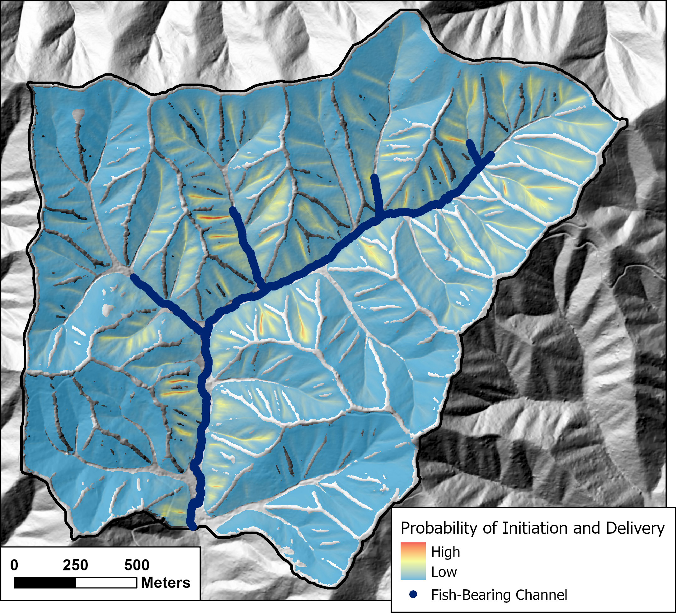
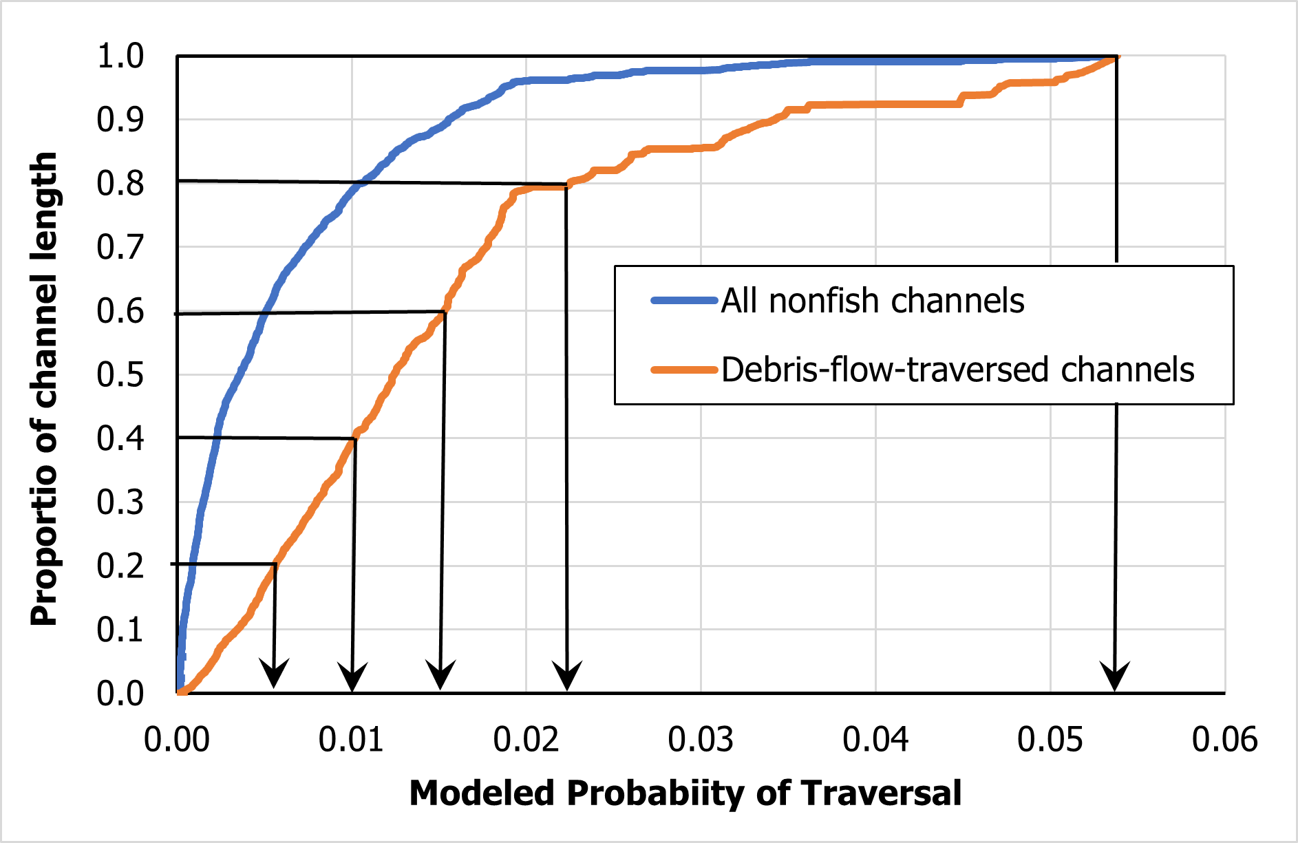
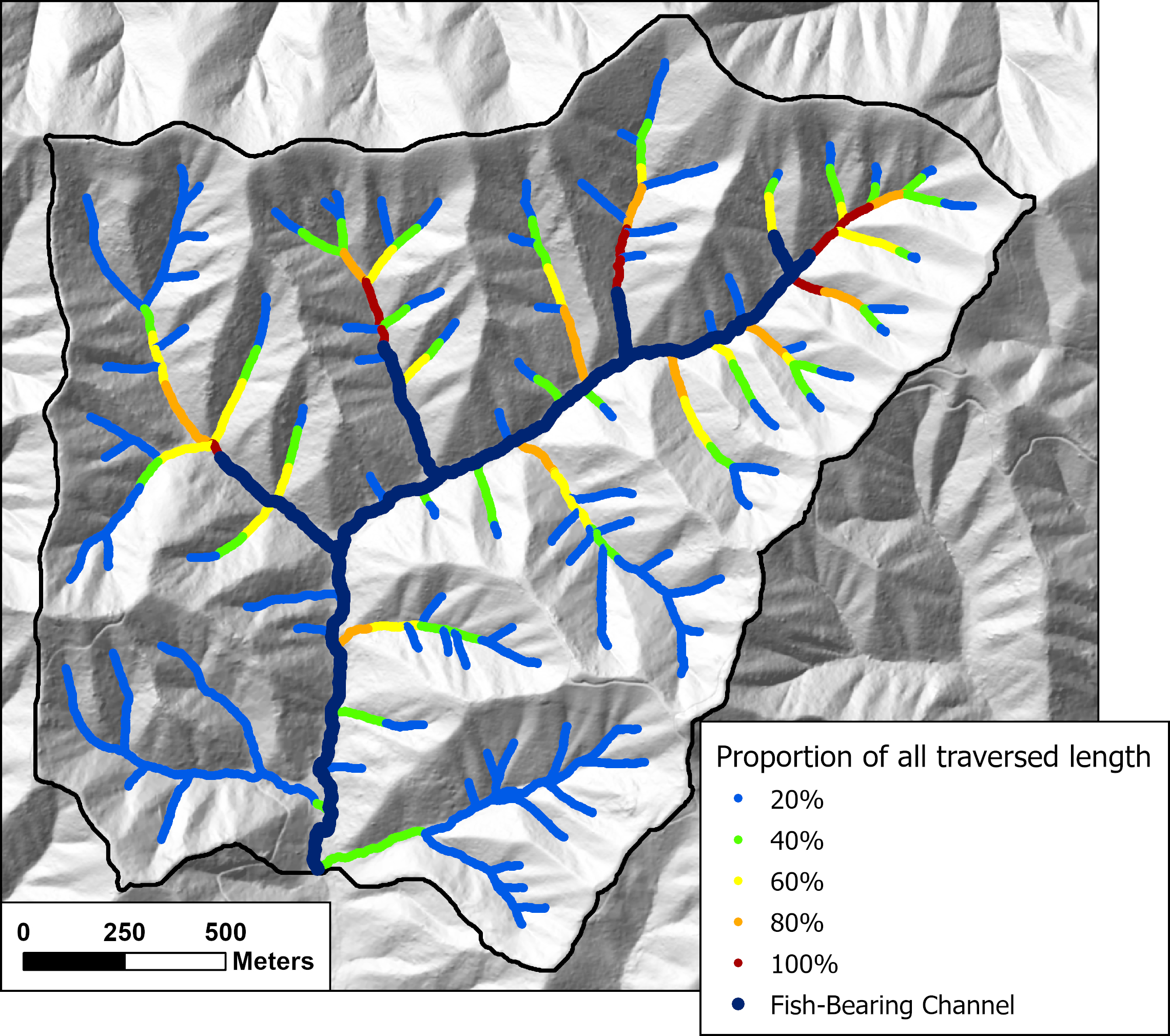
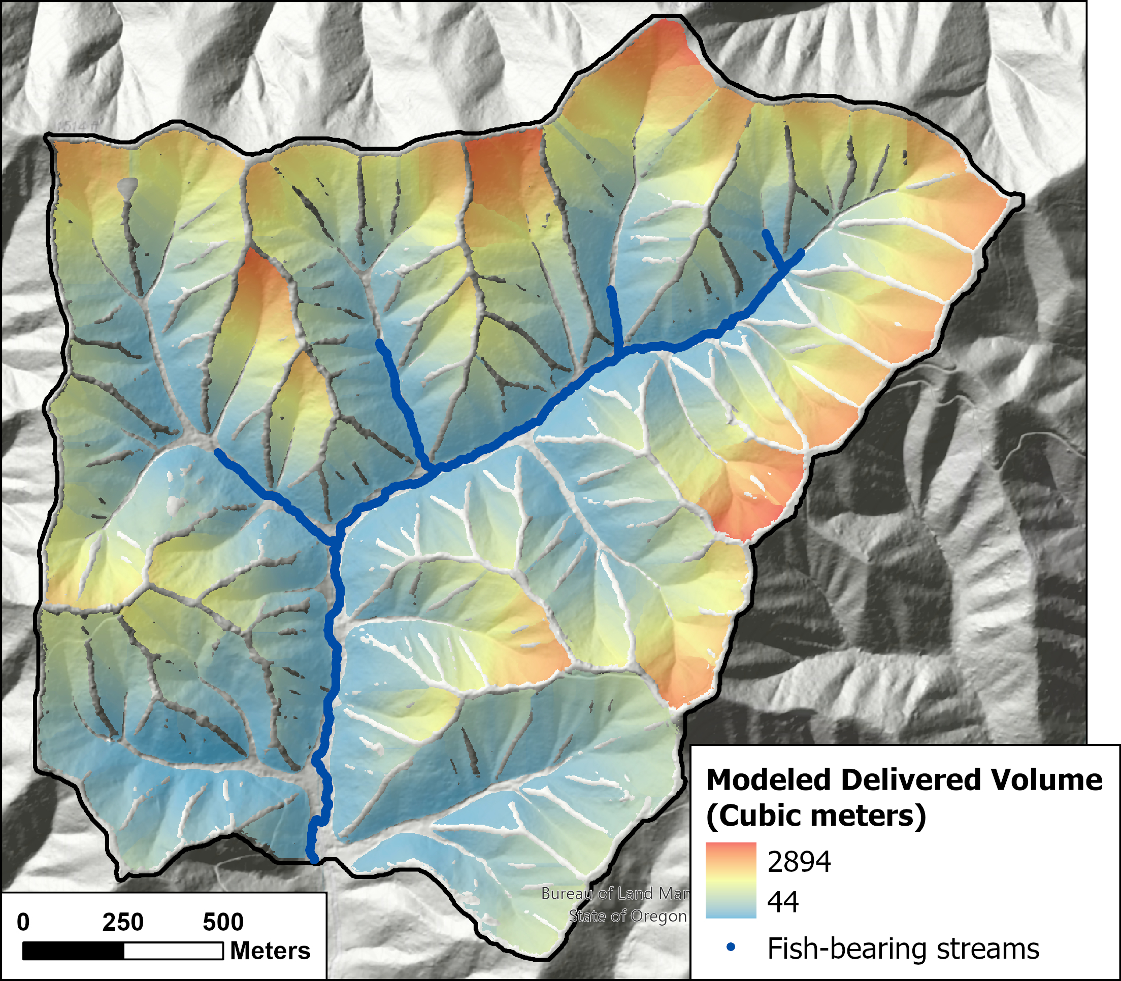
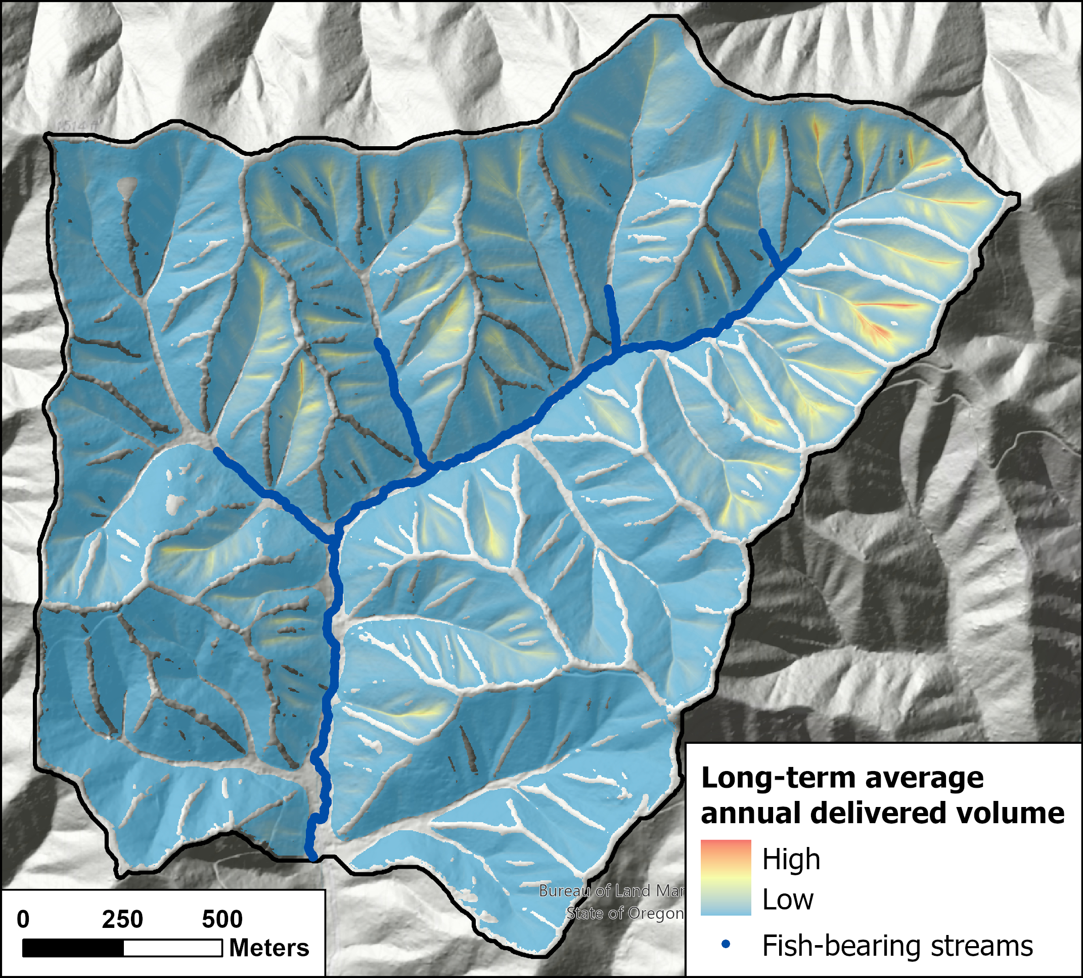
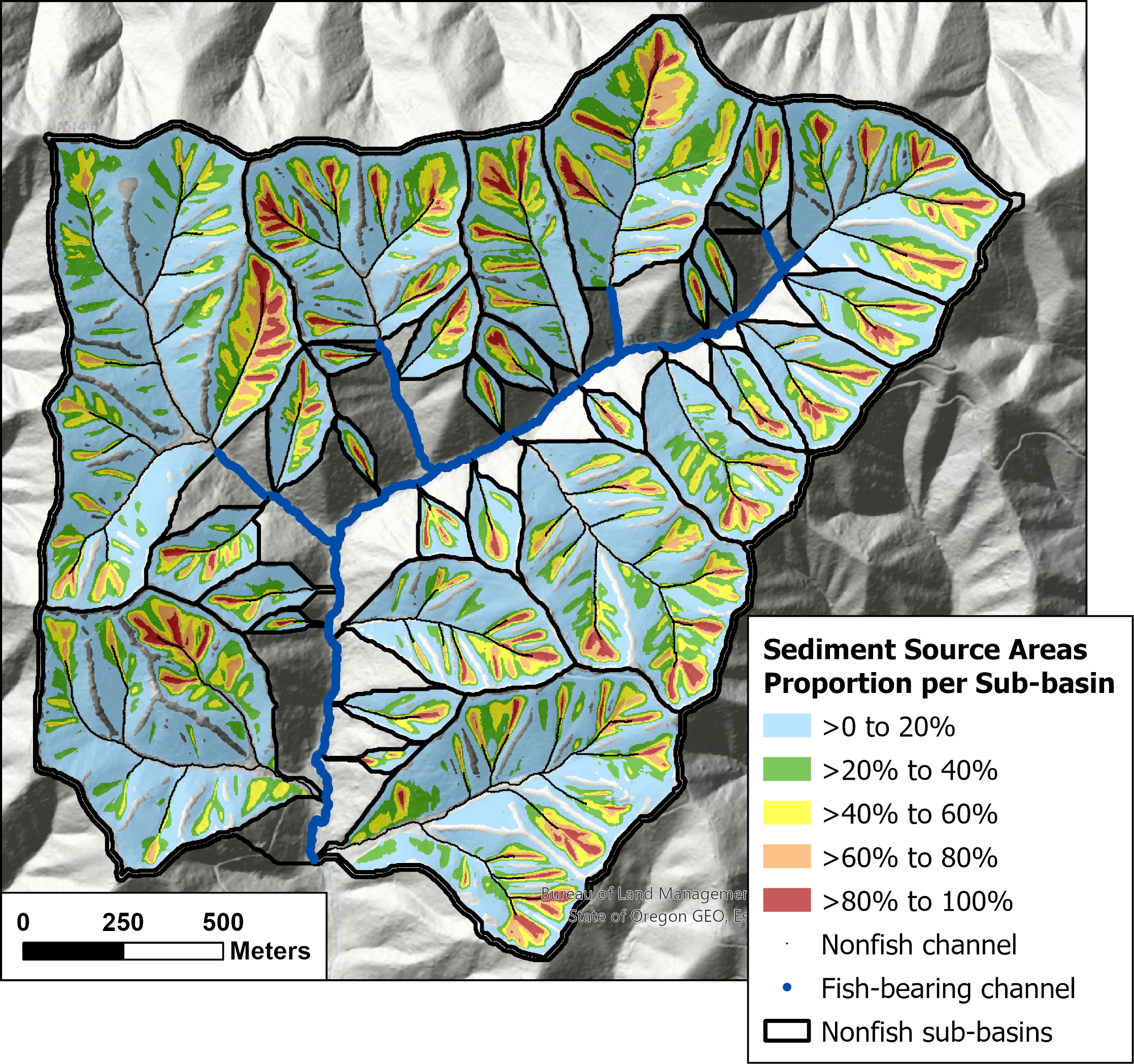
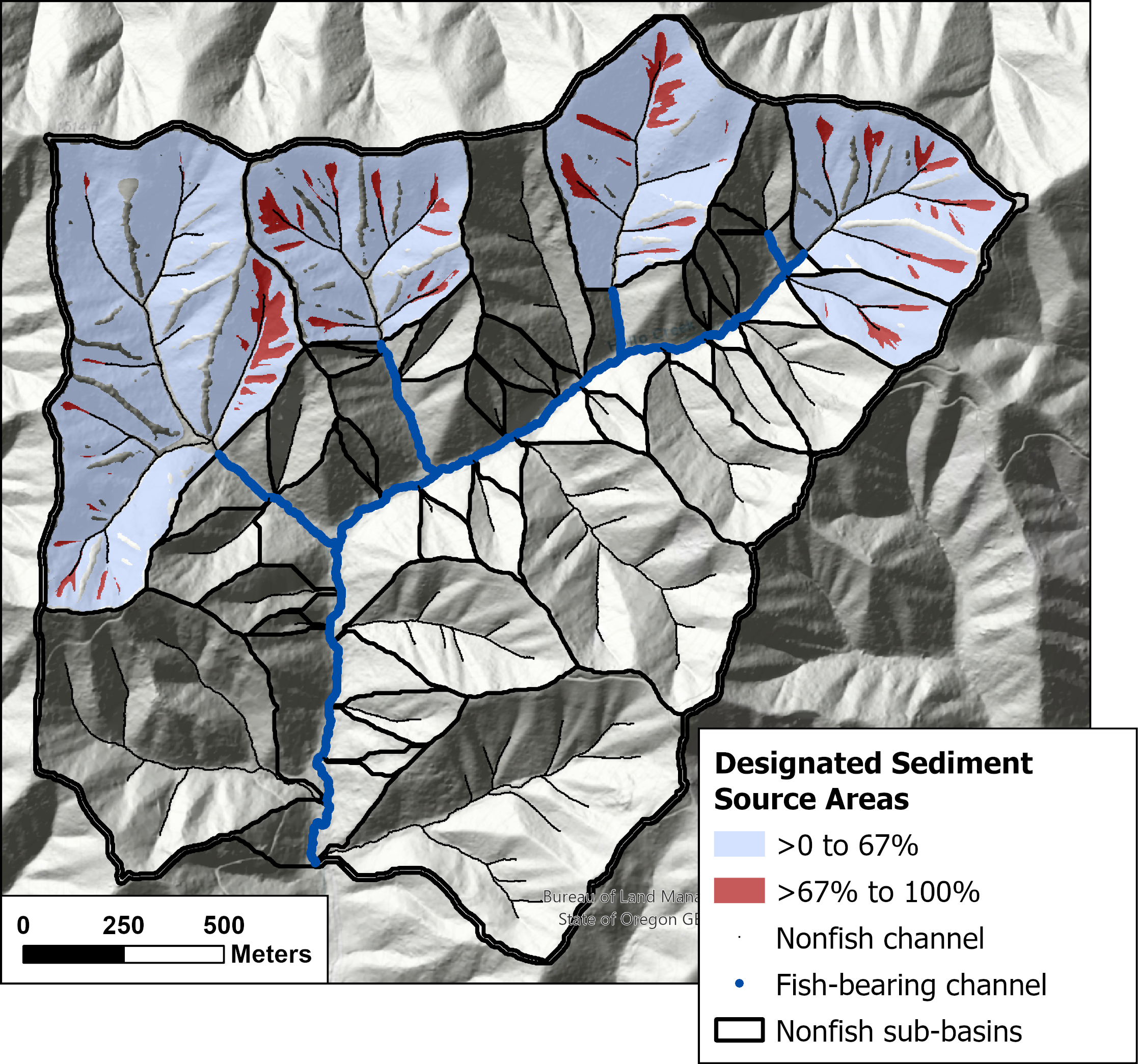
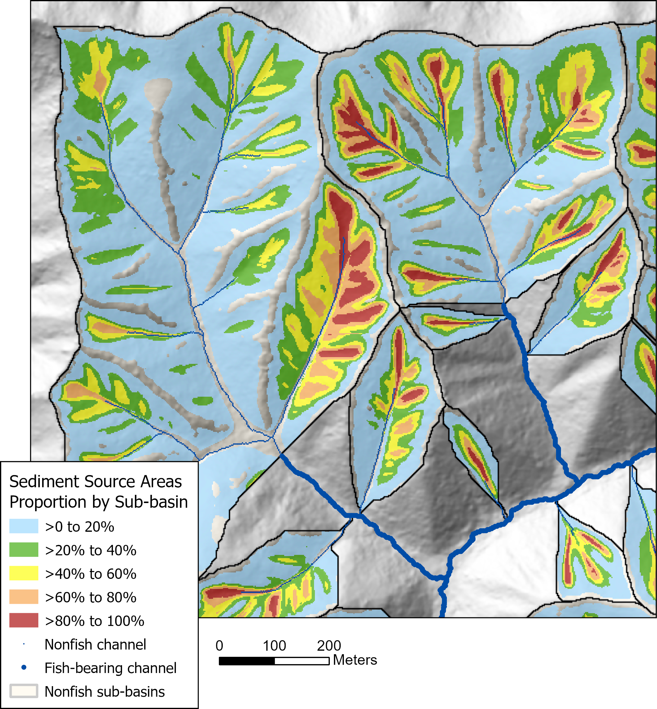
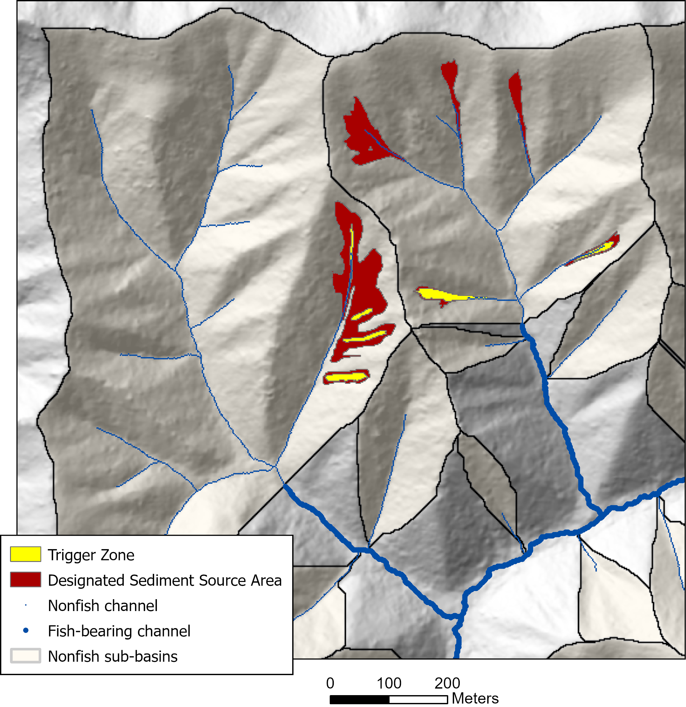
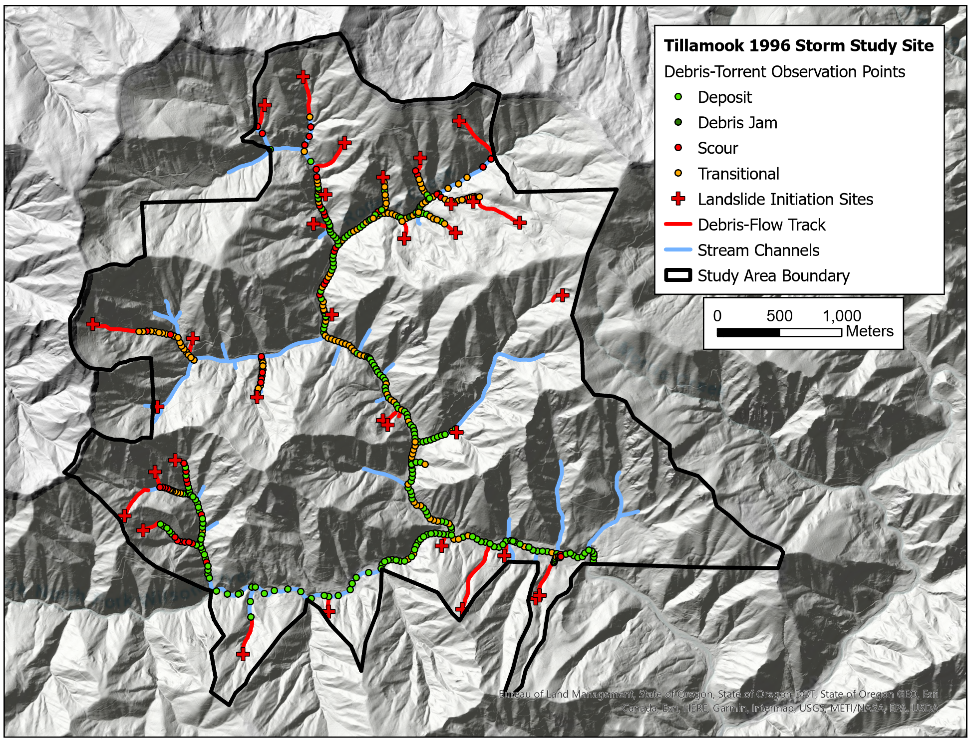
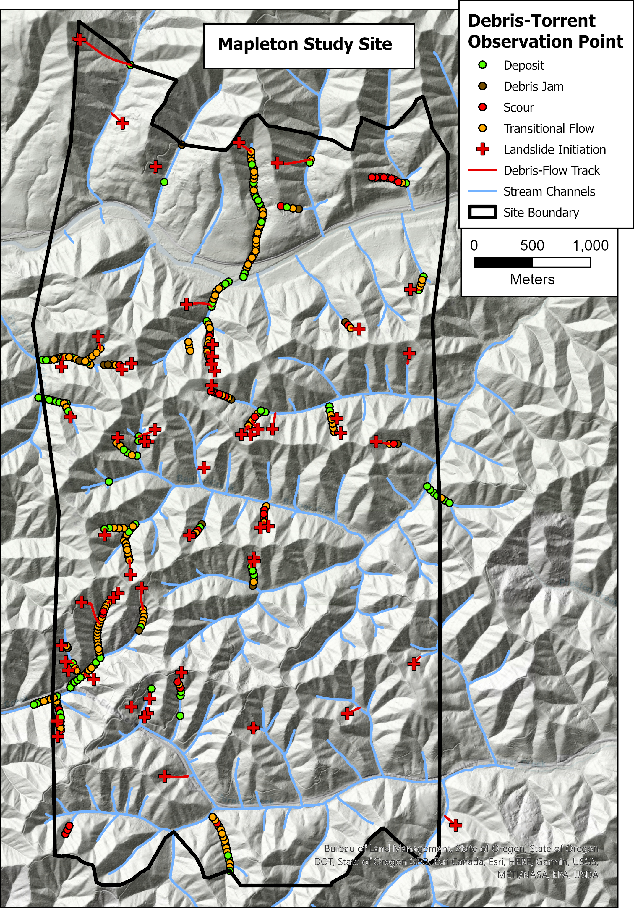
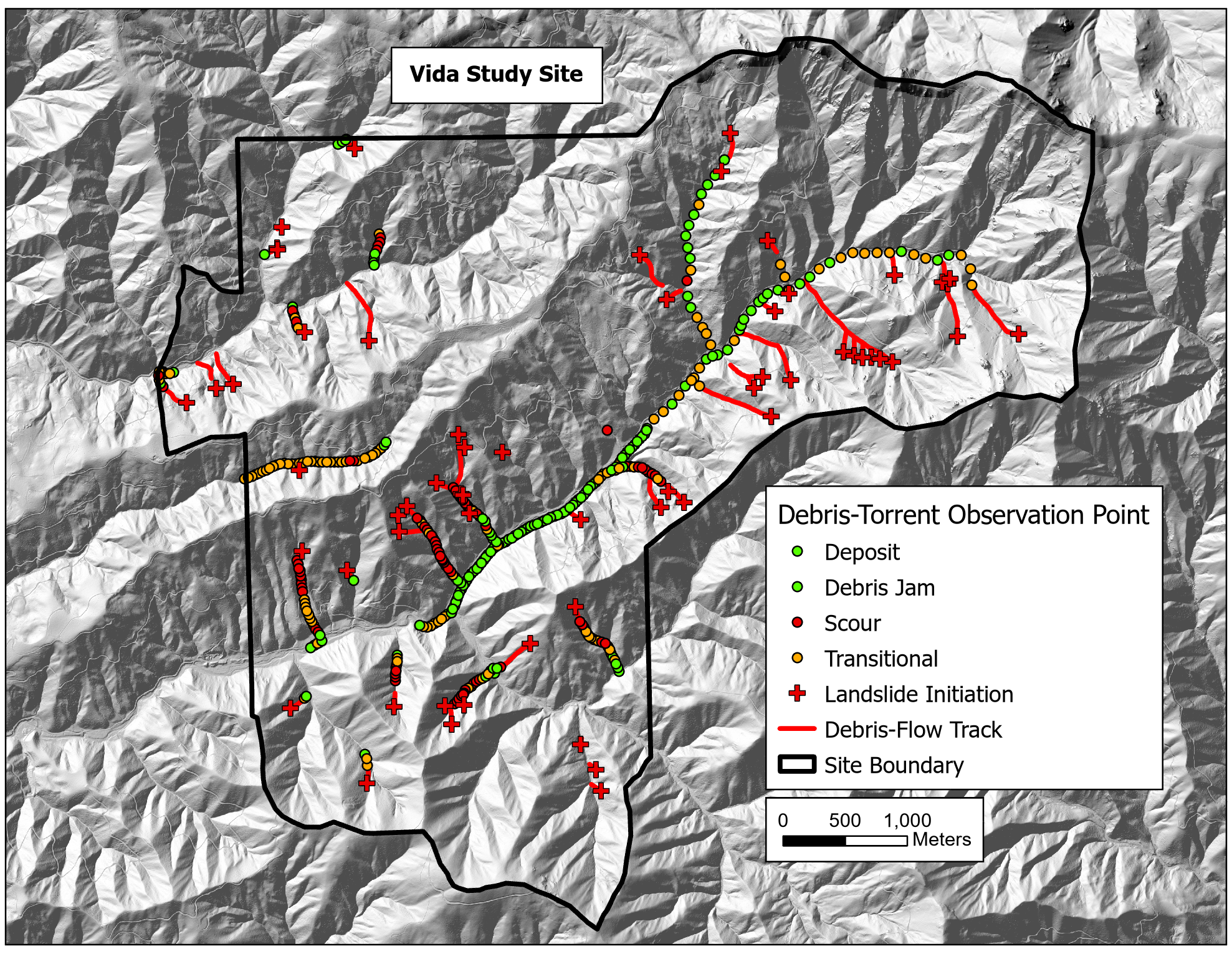
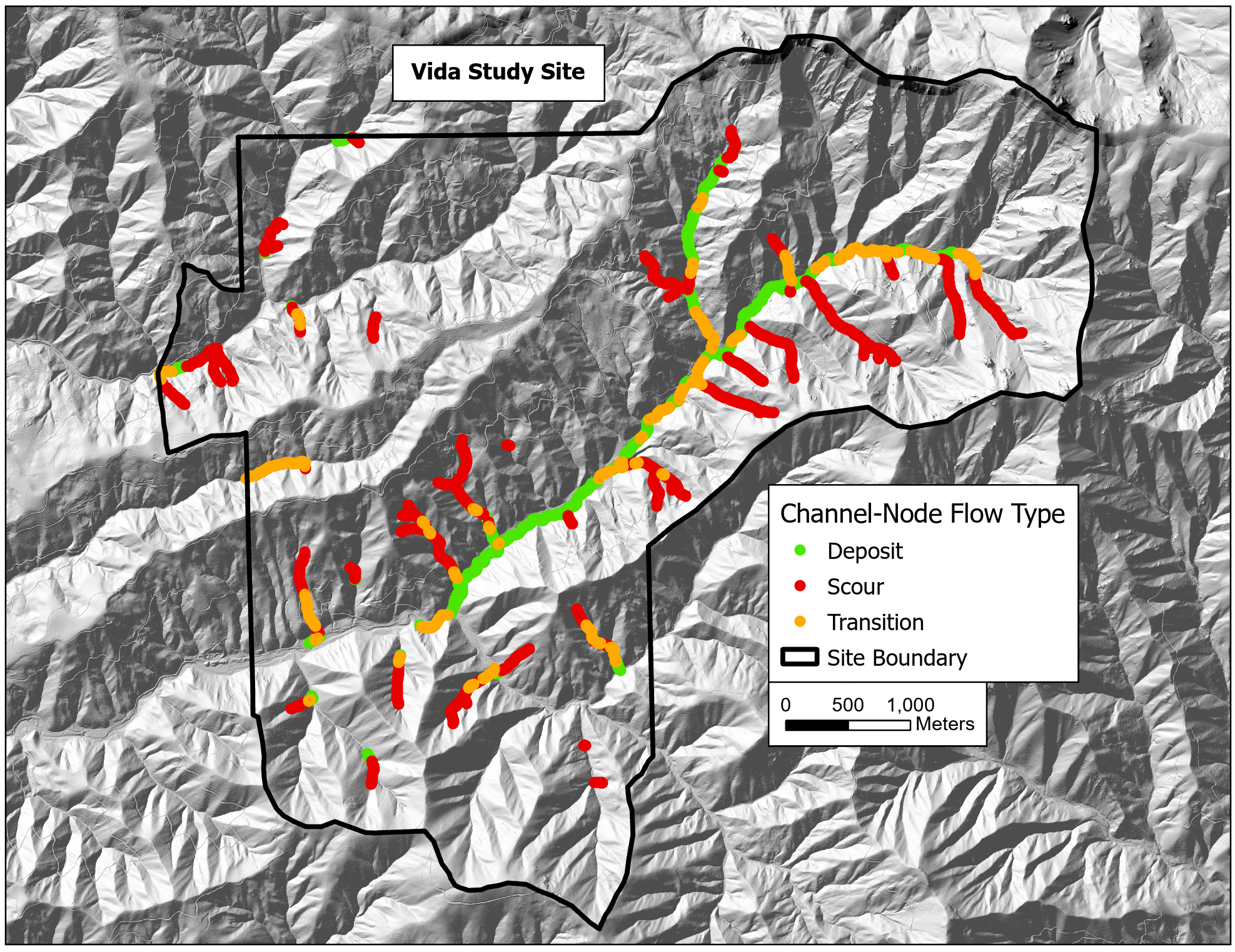
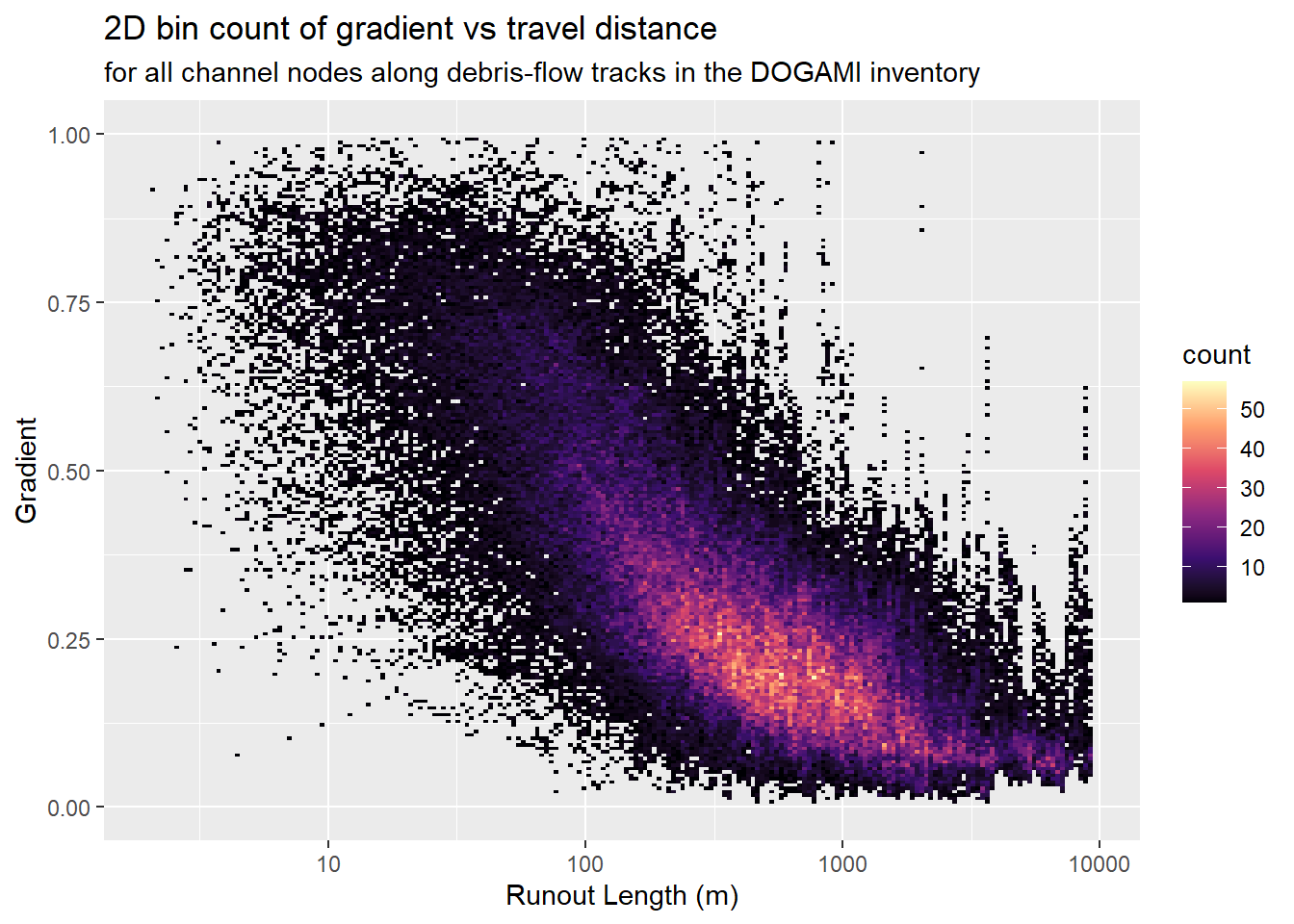
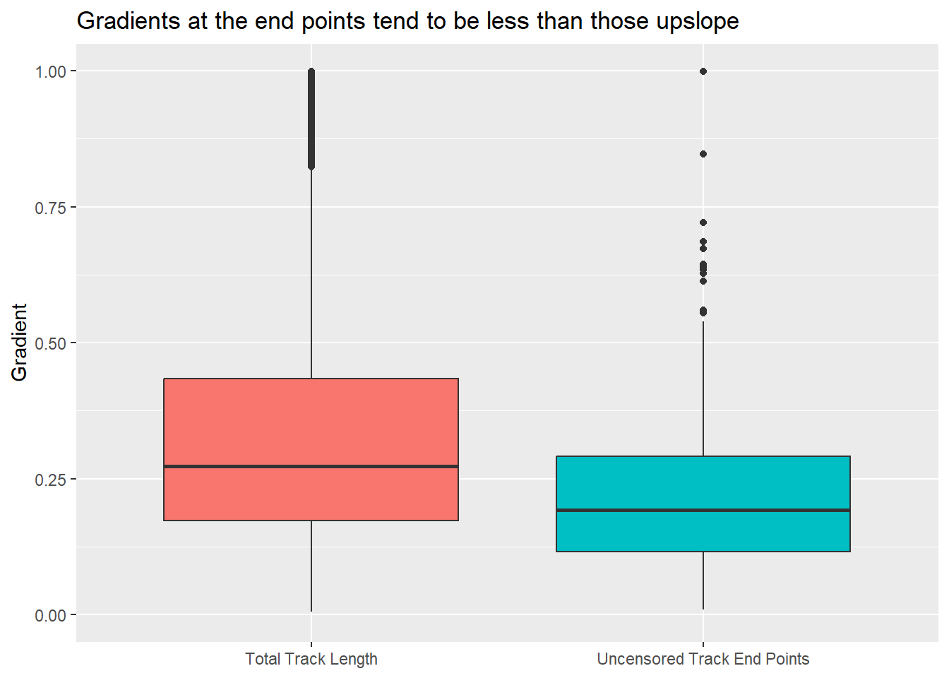
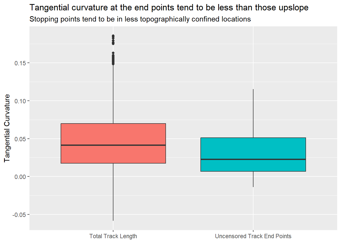
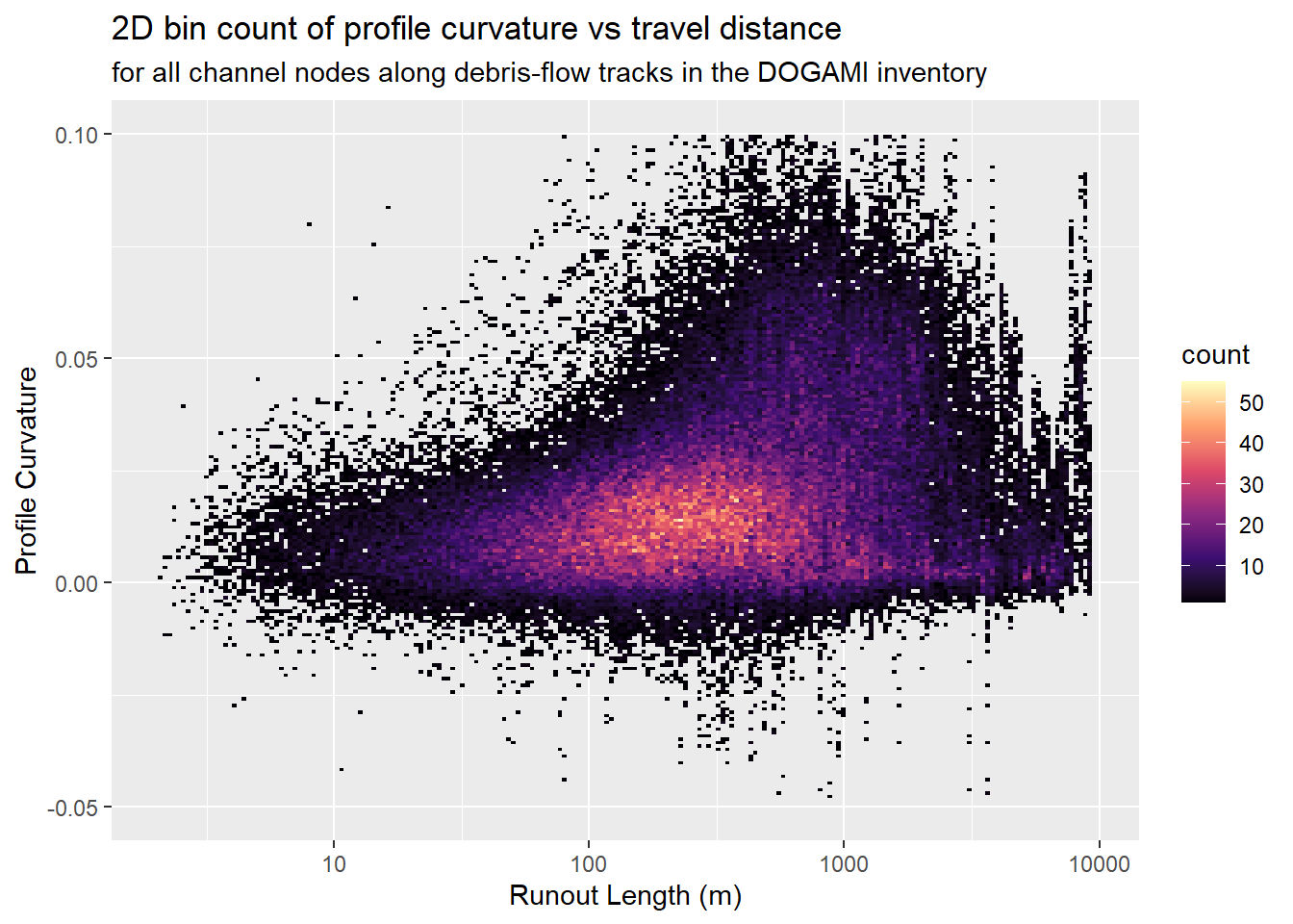
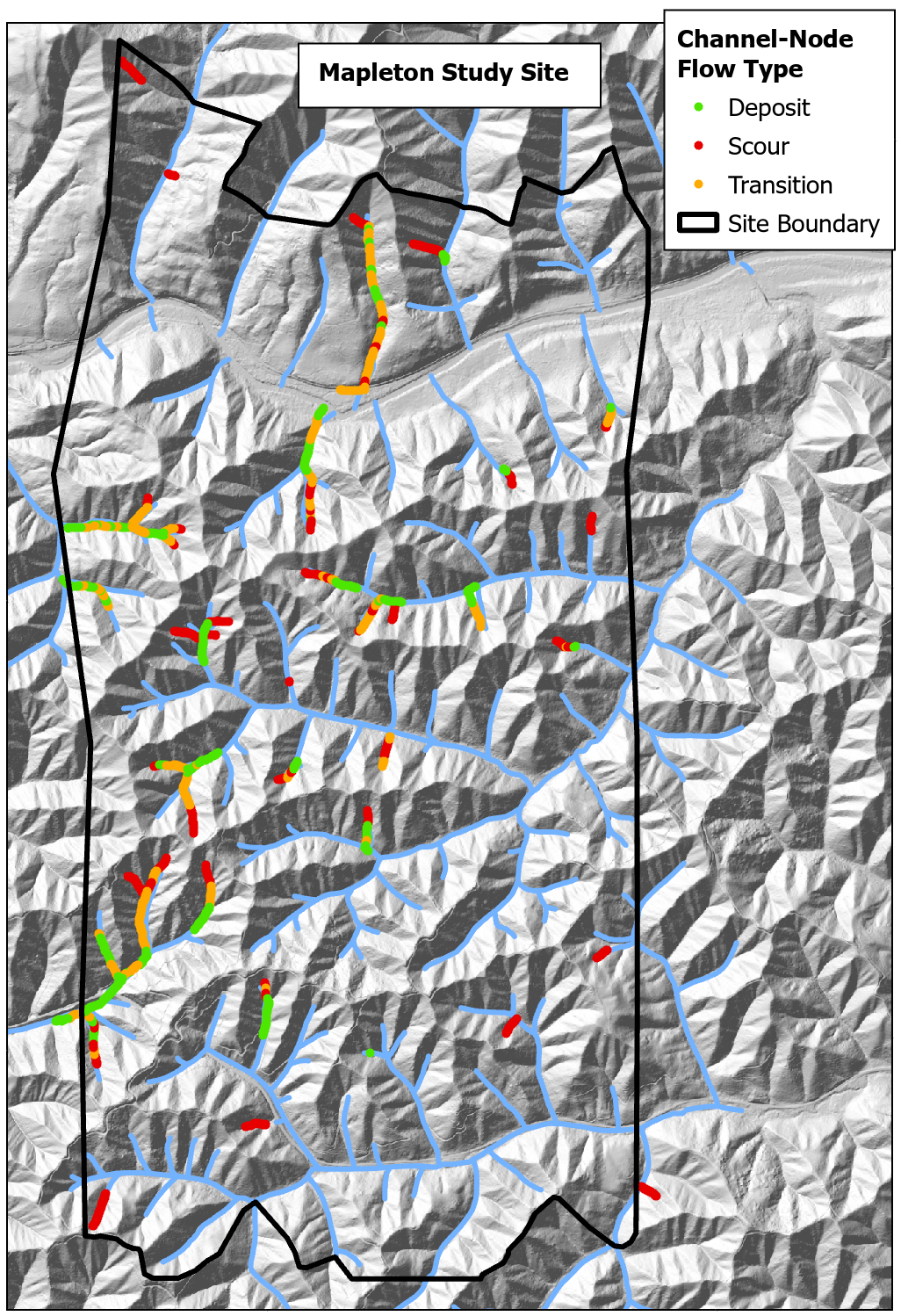