Steep-slopes modeling for the Private Forest Accord
1 Introduction
In steep-land regions of Oregon, landsliding of shallow soils that subsequently evolve into a debris flow are a primary process by which sediment and wood is carried from hillslopes to valley floors and stream channels (Swanson, Fredriksen, and McCorison 1982). The deposits formed by these events profoundly influence valley floor and channel morphology (L. Benda 1990; Bigelow et al. 2007). At any single failure site, the frequency of such events is rare, with recurrence intervals spanning thousands of years (L. E. Benda and Dunne 1987). There are many such sites, however, so when integrated over a channel network, these landslides and debris flows are important drivers of the disturbance regime that acts, in part, to set the spatial and temporal distribution of habitat types across a basin (L. E. Benda et al. 1998; Rieman, Dunham, and Clayton 2006). A goal of forest management is, therefore, to avoid doing things that will change that disturbance regime (Penaluna et al. 2018). This is reflected in the Private Forest Accord’s approach to timber harvest on steep slopes (Chapter 3 and Appendix B, Oregon Department of Forestry 2022), for which harvest prescriptions apply to the source areas and traversal corridors of debris flows that might travel to fish-bearing streams. These zones are ranked by the frequency of debris-flow delivery to fish-bearing streams, so that prescriptions can target those zones where timber harvest is most likely to alter the frequency and magnitude of sediment and wood fluxes to those streams.
These source areas and transport corridors are identified for the PFA using models of landslide initiation and debris-flow runout developed by Kelly Burnett and myself with the Coastal Analysis and Modeling Study (CLAMS) as described in Miller and Burnett (2007, 2008) with application of the models described in Burnett and Miller (2007). The original models were calibrated using landslide-initiation locations, debris tracks, and “debris-torrent”-impacted channels that were field surveyed for the 1996 Storm Study by the Oregon Department of Forestry (ODF) (Robison et al. 1999) and digitized to 10-meter line-trace DEM base maps. Several factors motivate a re-calibration and re-examination of these models.
Recent work by the Oregon Department of Geology and Mineral Resources (DOGAMI) (Special Paper 53, Burns, Franczyk, and Calhoon 2022) now provides an inventory of landslide initiation points and debris-flow-runout tracks with a greater geographic and temporal range than available from the 1996 Storm Study,
high-resolution DEMs derived from lidar are now available for much of Oregon (https://www.oregongeology.org/lidar/), and
statistical methods and analysis tools have progressed considerably in the last 15 years.
The Miller-Burnett models identify the channels susceptible to direct impacts from debris flows originating upslope and delineate the source areas for those debris flows. Although the initiation and evolution of a landslide into a debris flow is a continuous process, the models examine landslide initiation and runout separately. This is because initiation and runout involve different sets of physical processes influenced by different sets of environmental factors. An empirical approach is used for both cases, in which statistical models are calibrated using observed landslide initiation sites and debris-flow tracks, but with the choice of explanatory variables (also called the independent variables or predictors) based on current understanding of the physical processes involved. The models are linked in that the modeled potential for downslope impacts is a function of both initiation probability and runout probability. This document focuses on landslide initiation; a separate document describes the analysis done for debris-flow runout and subsequent analyses that utilize the linked models.
In the realm of forest practices, determination of hazards related to landsliding and debris flows has traditionally relied on field observations and mapping done by experienced professionals. Oregon, for example, provides guidelines for identifying and rating areas susceptible to shallow, rapidly moving landslides (Forest Practices Technical Note Number 2 and Number 6). Washington state provides guidance in the Forest Practice Board Manual (Section 16, Guidelines for Evaluating Potentially Unstable Slopes and Landforms). At one point, Lee Benda, I, and several others offered training for field identification and mapping of landslide hazards (Slope Instability and Forest Land Managers).
So why use a computer model now? Timber-land management seeks to promote both ecologic and economic integrity. Decisions about how to do that in the context of landslides and debris flows invariably involves trade offs between the extent of area where harvest restrictions apply and the area available for timber production. A method or model to quantify those trade offs can provide cost-benefit comparisons to inform decision makers. Once those decisions are made, a consistent method for mapping those areas across landslide-prone regions of Oregon is needed so that timber-land managers can incorporate that information into harvest and road-construction planning and anticipate the consequences for field operations. A computer model can provide a quantitative and consistent method for that mapping. The resulting maps are not necessarily better than those provided through manual mapping; indeed, ground-based observations will still be essential for the final determination of landslide-prone zones because many factors that influence landslide potential cannot be resolved from the remotely sensed data used by computer models. Several factors, however, render a computer model well suited for this task:
Manual mapping is subject to the experience and biases of the mapper, so different mappers produce slightly different maps. A computer model can provide a consistent result.
Manual mapping requires experienced professionals and takes considerable time and effort. A computer model can provide results for the entire state in a matter of hours. However, development of the model takes considerable time, effort, and expertise.
A computer model can incorporate information that is unavailable or difficult to measure through field observations alone. This includes such things as the upslope area contributing shallow subsurface flow for storms of variable duration or the cumulative length of scour zones along all potential upslope debris-flow corridors.
A computer model can be designed to make quantitative predictions of probability. Traditional field mapping may offer estimates of high, medium, and low potential, but cannot provide measures of probability. Comparisons of the costs and benefits of different options requires quantitative estimates of the consequences associated with those options, which requires quantitative estimates of the probability of the different potential consequences.
These models are empirical, in that they seek statistical relationships between observed landslide initiation locations and debris-flow corridors with topographic, geologic, and land-cover attributes. Given the large area over which the models must be applied, we use attributes that can be mapped remotely. Modeling strategies span a range from purely physically based (or process-based) models; those based solely on physical explanations of the phenomena modeled (landslide initiation and debris-flow runout), to purely empirical models, based solely on observed associations (locations of landslide initiation sites and channels traversed by debris flows with topographic, geologic, and land-cover attributes). In practice, physical models tend to include empirical components, and likewise empirical models may include and be guided by the underlying physical theory. That is true here; we use the conceptual physics of soil failure to guide our choice of topographic, geologic, and land-cover attributes to compare with landslide and debris-flow locations.
There are physically based models that could be applied here. SHALSTAB (Montgomery and Dietrich 1994; William E. Dietrich, Bellugi, and Real de Asua 2001), for example, could be used for landslide initiation and a model like D-Claw could be used for runout (see also Iverson 2014). There are several reasons we chose an empirical approach.
With a physically based model, we need to know the physics of what is occurring. There may be things occurring that we do not know about and would not, therefore, be included in a physically based model.
Physically based models incorporate simplifications and abstractions of the actual phenomena. This is intrinsic in development of mathematical descriptions of physical phenomena. SHALSTAB, for example, assumes steady-state rainfall onto a planar slope with uniform soil depth; simplifications of actual time-varying rainfall onto slopes with a great deal of topographic convergence and divergence and variable soil depths. This simplification allows for a concise mathematical description of soil failure with which predictions of where landslides are likely to occur can be made, but it will also result in inaccuracies in those predictions.
Physically based models require quantitative details about environmental attributes for which we have no information, such as spatial variations in soil depth and texture and the time series of rainfall. Application of these models then requires assumptions about these attributes, which will again result in inaccuracies in model predictions.
For these reasons, physically based models are often used to test and improve our understanding of the physics involved. Errors in predictions point to missing components in the model, or over simplification, or incorrect assumptions. Physically based models are also useful for anticipating the influence of different components in the model. For example, SHALSTAB has been used to show how loss of root strength associated with timber harvest might affect the area subject to landslide initiation (Montgomery, Sullivan, and Greenberg 1998). To evaluate effects of root strength with an empirical model requires extensive observations of landslide locations under different forest stand conditions and, even if a correlation is found, we would still be uncertain about the actual cause. But to know if predictions of a physical model are correct or not requires the same data. We need some measure of reality to compare to model predictions, without which we have no idea how much confidence to place in those predictions.
Empirical models come with their own sets of strengths and weaknesses:
Empirical models can provide useful prediction even if our understanding is incomplete or the information available is insufficient to fully characterize the processes occurring. For example, to determine the forces acting on a column of soil on a hillslope to calculate the potential for it to fail we need to know the soil depth, but we have no way to actually measure soil depths over regional extents. However, field studies find that soil depths vary systematically with topographic attributes of slope and curvature. These are quantities that we can measure over regional extents using digital elevation models (DEMs) and correlations are found between these topographic attributes and landslide locations. Even though we have not actually measured soil depth, these correlations provide a way to predict where landslides can occur.
An empirical model sees only what the data provided it offers. We seek correlations between inventories of mapped landslide locations with environmental attributes. If those inventories provide an incomplete or biased sample of where landslides can occur, then the resulting model will be incomplete or biased.
To estimate the effect of incomplete or biased data on predictions of an empirical model, a model can be trained (calibrated) with a portion of the available data and the predictions of that model then tested (compared) against the remaining data. The size of the prediction error on that test portion of the data provides an estimate of model sensitivity to the sample of landslide sites used to build the model. Current analysis protocols repeat that procedure many times using different subsamples for training and testing the model in each iteration. The range of prediction errors provides a measure of model sensitivity with which to gauge the confidence to place in predictions made for locations where landslide inventories for testing the model are not available.
The statistical methods used for empirical models use mathematical representations of the relationships between variables. The coefficients for those mathematical equations are adjusted so that the predicted relationship matches the observed relationship as closely possible. For example, we may use a linear equation to relate slope gradient to landslide density. We then adjust the coefficients for that equation to minimize the difference between the predicted and measured densities. The ability of that model to then predict actual landslide densities depends on how well a linear equation represents the actual relationship.
We must chose what variables to include in an empirical model. If the variables we chose have strong correlations with landslide location, then an empirical model can work well for predicting where landslides will occur. We therefore strive to include all variables that might correlate with landslide locations. There is also the potential for spurious correlations. A model trained to match random errors or noise in our data might appear to perform well on the training data but will do poorly at predicting landslide locations elsewhere. Separating the signal from the noise inherent in all data sources can be difficult; understanding of the physical basis of the phenomena can guide the choice of variables and mathematical equations used to characterize relationships between variables.
The statistical methods used for empirical models can provide a measure of probability. This is the primary reason that we use empirical methods for the steep-slopes analyses performed for the PFA.
Physically based and empirical models are not mutually exclusive. We incorporate elements of both in this analysis. We use the conceptual models on which physical models are built to guide our choice of explanatory variables and we incorporate predictions of a simple physically based model for water flux through hillslope soils as an explanatory variable.
2 Landslide initiation.
2.1 Quantitative measures of susceptibility.
For the PFA, we seek to identify source areas and traversal corridors for debris flows that carry sediment and wood to fish-bearing streams and to rank these by the relative frequency of debris-flow occurrence. To do that, for each point on a hillslope, we need to determine the probability for initiation of a debris-flow-triggering landslide and the probability that the subsequent debris flow will travel to a fish-bearing stream. In this document we focus on the probability of initiation; analysis of runout is addressed in a separate document. For this task, we do not need to know anything about when landslides will occur, only where they originate and the relative frequency with which they occur. We use an inventory of mapped landslide locations to do this. Landslide density, the number of landslides per unit area, provides an indicator of where landslides are more or less likely to occur. Higher density indicates higher probability of occurrence. If we observe that landslide density varies with topographic, geologic, and land-cover attributes; statistical methods can be used to build empirical models that specify landslide density as a function of those attributes. Multiplying density by area gives number of landslides; for a DEM cell, multiplying density by cell area gives the probability that a DEM cell contains a landslide initiation point from the landslide inventory. Empirical models that show how attributes of topography, geology, and land cover relate to landslide density thus translate directly to the probability that a DEM cell contains a landslide initiation point. Summing that probability for all DEM cells spanning the study area will return the number of observed landslides. Our goal then is to find models that resolve correlations between landslide density and mapped landscape and environmental attributes.
Landslide inventories show us where landslides occur and we use landslide density determined from these inventories as a measure of the likelihood of finding a landslide. To determine how frequently landslides occur requires measures of landslide rate: number per unit area per unit time. Direct measures of rate requires landslide inventories that span not only large areas but also long time periods. Available inventories do not span sufficient time to make reliable measures of rate. Instead, we use landslide density as an indirect measure of rate. An inventory shows how many landslides occurred over some finite period of time. If the spatial variation in landslide density is constant over time, then a one-time measure of that spatial variation is proportional to the spatial variation in landslide rate. We can infer spatial variations in landslide frequency directly from spatial variations in landslide density. If, however, relative differences in density change over time - if, for example, different storms tend to trigger landslides in different types of locations - then we need an inventory that spans sufficient time for a representative sample of storms to occur. The inventories collected by ODF for the 1996 storm study indicated how many landslides occurred during the February and November storms in 1996. The models built using that inventory (Miller and Burnett 2007, 2008) reflect the landslide locations associated with those storms. We do not know if different storm events would produce different patterns in the spatial distribution of landslides. The DOGAMI inventory in Special Paper 53 includes landslide events over a longer time span, from 1996 to 2011. This samples a larger range of storm events over a larger geographic area, so it should provide a more representative sample of where landslides occur in Oregon than the 1996 Storm-Study inventory.
A variety of statistical methods can be used to find associations between landslide density and landscape attributes. In our 2007 study (Miller and Burnett 2007), Kelly and I used the “frequency ratio” method, which estimates the change in area and the change in the number of landslides associated with some small change in the attribute of interest. This gives landslide density directly. Classification methods can also be used. These methods seek to classify any location as to whether it is or is not a landslide initiation point. This classification is based on the modeled probability: a probability greater than some specified threshold (e.g., 0.5) is classified as an initiation point. We are interested in the modeled probability, not the classification. Commonly used classification models include logistic regression, random forest, and support vector machines. For any set of attribute values, these models estimate probability as the proportion of sampled sites that contain initiation points included within the data space local to those attribute values.
Within any study area, landslide initiation points occupy a very small proportion of the total area. Consider a 10 km2 study area with an average landslide density of 1 landslide/km2 (10 landslides total). Using a 1-m lidar-derived DEM, there would be 10 DEM cells with landslide initiation points out of 10 million total cells. Calculations using such an unbalanced sample may reach the limits of computer precision; hence subsamples of the non-initiation DEM cells are typically used for analysis of landslide susceptibility. Because probability is based on the proportion of the total sample composed of initiation points and the number of initiation points is set by the landslide inventory, the modeled probability is proportional to the number of nonlandslide points included in the sample. This is not a problem if the sampled points are representative of the range of conditions over the study area: we are interested in the spatial variation of probability, not the magnitude. If we had a larger landslide inventory, for example, with twice as many landslide points over the same study area, landslide densities and modeled probabilities would be twice as large. Likewise, changing the balance of the sample between landslide and nonlandslide points will change the magnitude of the modeled probability, but as long as the samples are representative of conditions over the study area, that will not change the spatial pattern of relative changes. For the PFA analyses, we ultimately translate modeled probabilities to proportions of landslide and debris-flow events, and these proportions are not affected by uniform changes in probability.
We use logistic regression to model initiation probability. The frequency ratio used in the original model works well for one variable, but classification methods are better suited for multiple variables. Logistic regression is more easily interpreted and understood than the other classification methods.
2.2 Predictors
There are several things to consider when choosing predictors to include in an empirical model:
Which landscape attributes are related to landslide density? The ability of a model to resolve variability in landslide potential depends on the degree to which the predictors used in the model are systematically associated with spatial changes in landslide density. We do not want to exclude any potentially informative predictors, but inclusion of correlated, or uninformative, or biased predictors will negatively impact model performance. In a review of the literature, Lima et al. (2022) counted 116 different predictors that have been applied in empirical models for landslide susceptibility. Such latitude offers plenty of opportunity for wasting time. Our choice of predictors is guided by physically based models of soil failure.
Which attributes can be measured over the area of western Oregon where the model must be applied? Any predictors used must be obtainable from data sets with consistent state-wide coverage. Topographic attributes are calculated from lidar DEMs, which are available for almost the entire area. Datasets for substrate (geology) and land cover are available, but at lower spatial resolution than the DEMs.
At what spatial scale should the attributes be measured? The length over which measurements of landscape attributes can be made is constrained by the spatial grain of available data. Within those constraints, measurements should be made at length scales appropriate for the physical processes driving soil failure. Lidar DEMs provide point measures of elevation over approximately a one-meter grid spacing. Measures of topographic attributes can therefore be made from a length of several meters, spanning two to three DEM points, to any longer length desired. The value measured will vary with the length over which it is measured. Consider gradient: measurements over several meters will resolve the effect of tree-fall pits. Measurements over tens of meters will miss the pits, but will resolve changes in gradient associated with bedrock hollows. Measurements over hundreds of meters will resolve influence of large headwalls. A length scale that is too small will resolve changes in gradient not associated with landslide locations, thus adding noise to the data; a length scale too large will miss the topographic features associated with individual landslides.
2.2.1 Which Attributes?
Conceptually, soil on a hillslope will slide downslope when the gravitational force acting to move it downslope exceeds the forces acting to hold it in place. The physical details are complex, but geotechnical engineers have abstracted these details into relatively simple models that are remarkably successful at describing observed soil failures. These simple models guide our choice of predictors. The “infinite slope” model (Skempton and deLory 1957) is the starting point for many physically based models of soil failure, such as STALSTAB (Montgomery and Dietrich 1994). Forces are calculated for a column of soil overlying a competent substrate. The weight per unit area of the column (weight equals column depth times soil bulk density) times the sine of the slope angle gives the force acting to move the column downslope. Frictional resistance, intrinsic soil cohesion, and the network of plant roots connecting the column to the substrate act to hold the column in place. Water filling the void spaces between soil particles reduces frictional resistance to an amount proportional to the depth of saturation.
Even for this simple model, we cannot measure all the variables required to calculate these forces (soil depth, friction angle, cohesion, saturation depth), but we can measure the topographic and land cover attributes that influence these variable values. Slope gradient can be obtained directly from a DEM. Field surveys find that soil depth correlates with slope and topographic curvature (Patton et al. 2018). During a rainstorm, infiltrating water flows downslope through the soil layer. The volume of water flowing through a column of soil increases during the storm as infiltrating water from further and further upslope reaches the column. That volume is determined by the area from which infiltrating water reaches the soil column (the contributing area) and the rainfall intensity (depth per unit time). The contributing area, and the corresponding depth of saturation, increases during the storm at a rate dependent on rainfall intensity and upslope topography. The velocity with which water flows through the soil increases as slope gradient increases. We can use the spatial variation in upslope gradient and aspect to calculate the size of the contributing area to a column of soil over time. Spatial variation in contributing area translates to spatial variation in saturation depth (e.g., Iida 1999). Thus, based on this simple model, the spatial distribution of three topographic attributes is related to the potential for landslide initiation: slope gradient, curvature, and aspect. These can all be calculated using a DEM.
Soil strength, in terms of frictional resistance and cohesion, are related to the texture (size distribution and shape of soil particles) and its mineralogy. These properties are in turn related to the type of rock the soil originates from. Spatial variation in rock type may thus also be related to spatial variation in landslide potential. DOGAMI provides statewide GIS data for geologic mapping (https://www.oregongeology.org/geologicmap/index.htm). This is a compilation of many different data sources.
The degree to which plant roots might act to anchor the soil to the underlying substrate and adjacent soil depends on the number and strength of those roots (e.g., Sidle 1991; Schmidt et al. 2001). Numerous studies have reported accelerated landslide rates after timber harvest (e.g., Swanston and Swanson 1976; WOLFE and WILLIAMS 1986) and reductions in harvest-associated increases in rate with changes in harvest practices (Woodward 2023). We can expect, therefore, that some measure of stand characteristics might be associated with landslide rate. In our analysis of the 1996 storm data, Kelly and I found an association with stand age (Miller and Burnett 2007). Turner et al. (2010) also found systematic differences in landslide density with stand age. Schmidt et al. (2001) warn that effective root strength may not uniformly improve with stand age, but we need to work with some measure of stand conditions that can be consistently measured over all of Oregon. The Landscape Ecology, Modeling, Mapping & Analysis project (LEMMA) provides stand-structure maps that include “Basal area weighted stand age based on dominant and codominant trees” for Oregon. There are a variety of other metrics available, but so far stand age is the only one we have evaluated. However, for the PFA analysis, we want to use predictors that do not change over time, at least over the time frame of a harvest rotation, so stand age is not included in the model used for PFA.
As mentioned above, soil depth is an important factor affecting failure potential. Another process that affects soil depth, particularly along the axis of a topographic hollow, is the frequency of debris-flow scour. Depending on storm characteristics, landslides may be triggered at different locations points up or downslope along a hollow axis (Dunne 1991). The subsequent debris flow can scour the downslope portion of the hollow axis to bedrock. Soil then accumulates within the scoured zone over time (W. E. Dietrich et al. 1982; May and Gresswell 2003) until, at some point, it is deep enough to fail again. A debris-flow triggered far upslope along a hollow axis will thus reduce the potential for subsequent landslides downslope for the time it takes soil to accumulate to sufficient depth to become unstable during a storm. Thus, the potential for landslide initiation along a hollow axis is presumably a function of the frequency with which it is scoured by debris flows. We cannot measure this frequency directly, but we might find a topographic proxy. The frequency of debris-flow traversal is a function of the number of upslope landslide sources. In steep terrain, the number of landslide sources increases with upslope contributing area. This refers to total contributing area, measured to the drainage divide, not that associated with a particular storm duration. Total contributing area can also be measured as a function of the upslope distribution of slope aspect, which we obtain from a DEM.
Forest roads alter hillslope topography, locally increasing slope gradient on cut and sidecast slopes and altering drainage patterns by redirecting surface and shallow subsurface flows of water. Both effects can change the potential for soil failure, so proximity to a road may also be associated with increases in landslide density, as found in numerous studies (Amaranthus et al. 1985; Gucinski et al. 2001; Miller and Burnett 2007). Distance to a road is an attribute we can examine, but because new roads are built and existing road conditions evolve over time, we will not include it in the model used for the PFA analysis.
2.2.2 Algorithms for Topographic Attributes
We identified slope gradient, curvature, and contributing area as potentially informative predictors for landslide density. These can be calculated from the gridded elevation data provided by a DEM. We must select the length over which these values will be measured and the algorithms for calculating those values (Newman et al. 2022). Both choices affect the degree to which the surface inferred from the elevation values is smoothed and the scale of landform features that can be resolved. Smoothing allows us to ignore both features too small to influence landslide potential and noise in the DEM data. Lidar DEMs are derived from the point cloud of reflections obtained from an aerial (airplane-mounted) laser signal. The point cloud includes reflections from the ground surface and the vegetation above it. For any signal, the reflection with the longest return time is interpreted as a ground return. The elevations of the ground-return points are then interpolated to a regular grid to produce a DEM. However, not all last returns are from the ground, some signals may not penetrate through the vegetation so the last return is above the ground. This results in a variable spatial density of ground returns and some reflections from vegetation incorrectly interpreted as ground returns. We want to measure gradient and curvature over a length scale sufficiently long that these errors will have minimum effect.
High-resolution lidar DEMs can potentially resolve features on the ground spanning only a few meters. This will include the head scarps and scars of the mapped landslides and debris flows in our landslide inventories. Our interest, however, is in the pre-failure topography; if the initiation point is associated with the gradient of the head scarp, we will over-estimate the gradient associated with that landslide initiation point. So we want to chose a length scale sufficient long to smooth out features like shallow-landslide headscarps, but still sufficiently short that the hollow the headscarp might be located in is well characterized.
To calculate elevation derivatives from a DEM requires that the shape of the ground surface be inferred from the grid of elevation points. Generally, a smooth surface is fit to the points in the neighborhood of a central point and gradient and curvature for that central point are obtained from the equation for that surface. Polynomial equations are typically used to describe that surface, from planar to third order (Florinsky 2016). The method used here is as follows. For each DEM grid point, elevations are obtained for the point and at eight equally spaced points along the circumference of a circle centered over that point. The diameter of that circle indicates the length scale of measurements. Elevations along the circumference are obtained using binomial interpolation from the four surrounding grid points. These nine elevation values are then used with equations derived by Zevenbergen and Thorne (Zevenbergen and Thorne 1987), modified for use with a circle (Shi et al. 2007). The resulting surface intersects those nine points and varies smoothly between them. Gradient, curvature, and aspect for the central point are then obtained from derivatives of the equation for that surface.
We used a circle diameter of 15 meters. This is short enough to resolve small hollows and swales and (we think) for measuring the degree of topographic confinement along debris-flow corridors. It is also short enough that a 2-meter headscarp will produce about a 10% change in measured gradient. We do not currently have an estimate of the degree to which post-failure topography biases measures of topographic derivatives associated with landslide initiation locations. We have not yet performed a detailed sensitivity analysis to examine this issue. With advent of landslide inventories based on lidar differencing (Bernard, Lague, and Steer 2021), this question can be addressed directly.
To calculate contributing area, the ground surface is parsed into square horizontal cells associated with each DEM point. The flow that surface water would take over the ground surface is then proportioned from cell to cell. There are a variety of algorithms for this (Wilson et al. 2008), of which D-infinity (Tarboton 1997) is considered one of the best performing (Riihimäki et al. 2021). D-infinity accommodates downslope dispersion by distributing flow to two of the downslope cells. Recursive iteration following flow paths through the DEM is then used to sum inputs from all upslope cells. The resulting contributing area to a DEM cell then indicates the cumulative area of all upslope cells that contribute flow to the cell. This contributing area also applies for water infiltrating the soil during rainstorms, assuming that flow through the soil follows similar flow paths as surface water. To calculate the area contributing shallow subsurface flow to a DEM cell during a rainstorm, we must account for the velocity with which water flows through the soil. This velocity is determined as the Darcy velocity \(V_D\)
\[ V_D = K\sin(\theta)\cos(\theta) \tag{1}\]
where \(K\) is the saturated hydraulic conductivity and \(\theta\) is the hillslope gradient. Equation 1 gives the flow velocity measured horizontally, assuming that the direction of shallow subsurface flow through the soil is parallel to the surface. Looking upslope from a DEM cell, we find which cells contribute flow to that cell and calculate the time for flow from the upslope to the downslope cell using Equation 1. This step is repeated moving upslope cell by cell until the cumulative travel time along a flow path equals the target duration. All the cells traversed then define the contributing area to the starting cell for that storm duration.
Saturated hydraulic conductivity for porous soils is on the order of one meter per hour (https://structx.com/Soil_Properties_007.html). Using that value, Figure 1 shows how the pattern of high and low contributing area changes over time. Each map shows contributing area in DEM cells with a linear color ramp scaled from a value of one cell (the minimum) to the mean plus one standard deviation in contributing-area values. This provides a consistent scale for visually comparing the results.
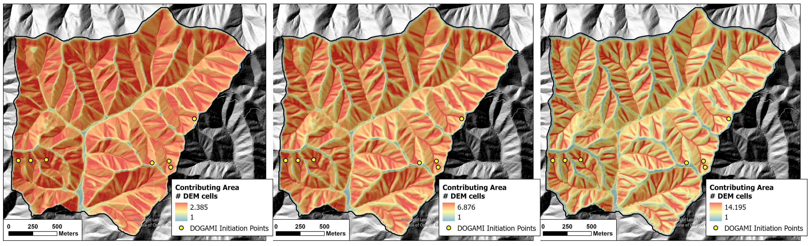
A high-intensity short-duration storm will produce similar levels of soil saturation across all hillslopes. As the level of saturation is a function of both contributing area and intensity, if the intensity is high enough to trigger landslides, these may occur over a broad area. During a longer duration storm, the highest levels of soil saturation become concentrated along hollow and swale axes. Thus landslides are more likely to be triggered in those zones. It is well recognized that landslide potential increases with increasing rainfall intensity (e.g., Turner et al. 2010); these results suggest that landslide locations may vary with storm duration. We use the calculated contributing area for several different storm durations as predictors for landslide initiation.
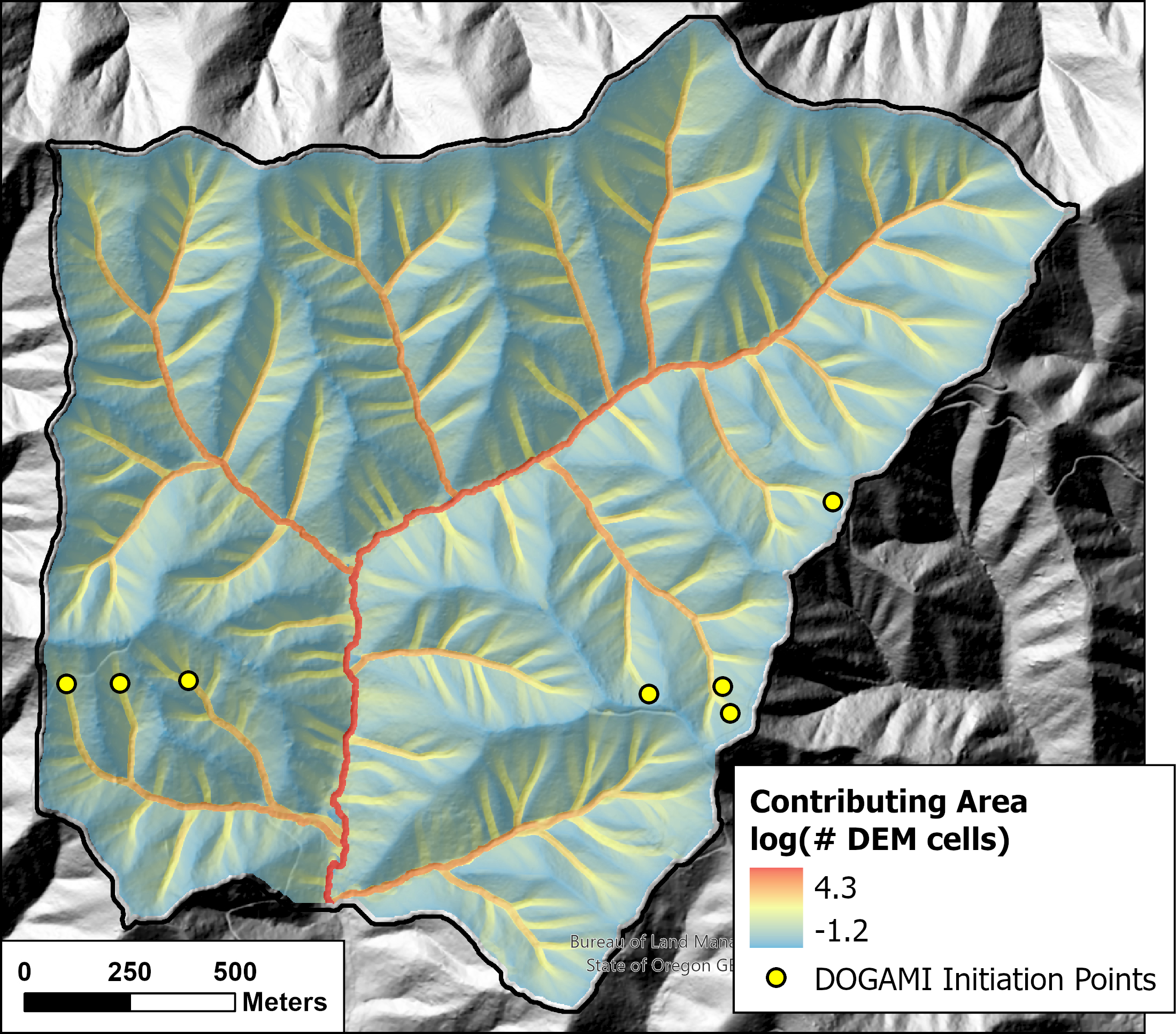
The total contributing area to a DEM cell, that which would occur during an infinite duration storm, is shown in Figure 2 below. This map shows the maximum contributing area within a 7.5-meter radius of each DEM point. The largest contributing areas are far larger than those illustrated in Figure 1 and increase monotonically downslope.
3 Data
3.1 DOGAMI inventory.
Landslide locations in the ODF 1996 Storm Study and DOGAMI Special Paper 53 inventories are shown in Figure 3 below. The 1996 inventory was based on field-based censuses of landslides within delineated study areas following storms in February and November. The DOGAMI inventory includes landslides associated with the 1996 storms, but also more recent events up to 2011.
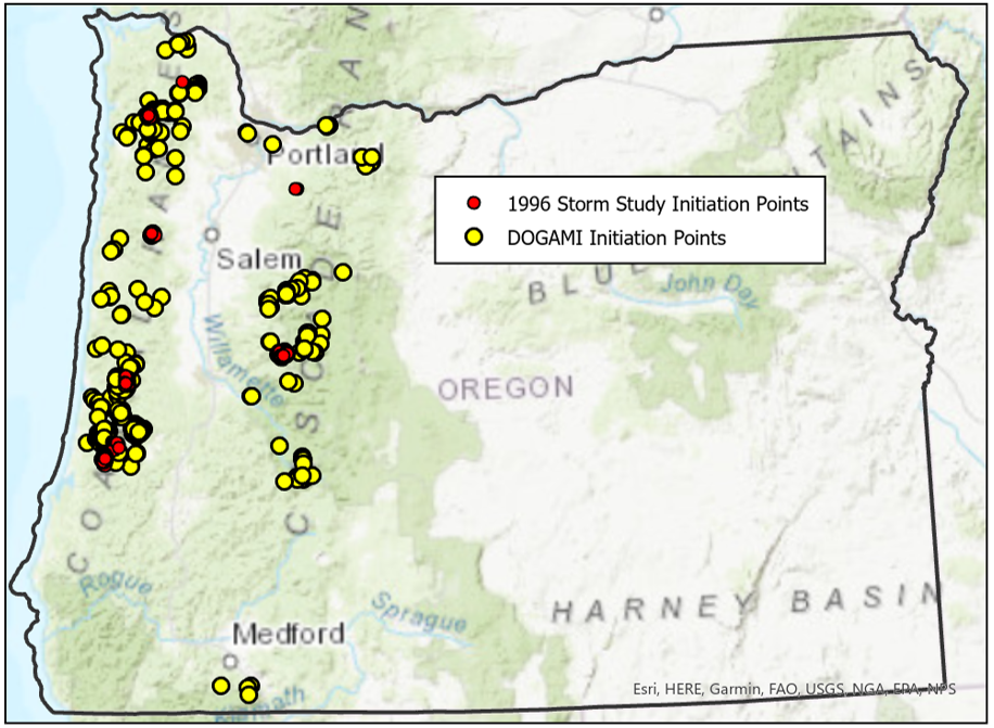
The DOGAMI inventory has more landslides than the 1996 inventory and it spans a larger geographic and temporal range. Hence, it should provide a better sample of conditions where landslides occur across western Oregon than available from the 1996 inventory. There are two factors to consider when using estimates of initiation susceptibility based on these inventories.
How well the inventory reflects the actual set of landslide scars and runout tracks that exist within the study area. Measures of susceptibility are based on measures of landslide density. Density is typically reported in terms of number per unit area, but may also be measured as landslide area or volume per unit area and as runout-track length per unit area or per unit channel length. If the inventory does not include all the landslides that exist within the study area, measures of density will be too small. If the missing landslides tend to occur in particular terrain locations, then resulting measures of spatial variation in landslide density and susceptibility will be biased. Inventories based on mapping of landslide scars from aerial photographs suffer from detection bias: small landslides and landslides under forest canopy are less visible than large landslides and those in clear-cuts and young forests. This results in bias with lower apparent densities measured in older forests. This bias can be substantial. With the field-based inventory for the Mapleton study area in the ODF 1996 Storm Study, Robison et al. (1999) found a 1.9-fold difference in landslide density (#/area) between young (<10 years, 21.1 landslides/square mile) and old (>100 years, 11.2 landslides/square mile) forest stands. Mapping done from 1:6000-scale photos found a 20.7-fold difference (12.4/sq mile for young stands versus 0.6/sq mile for old stands); mapping done from 2:24,000-scale photos found a 17-fold difference (5.1 versus 0.3 per square mile). The photo-based inventories indicated a difference in landslide density between young and old stands ten times greater than the field-based inventory. This detection bias hinders attempts to quantify associations of forest stand characteristics with landslide density. Furthermore, if stand characteristics vary with terrain location (e.g., if older stands tend to be located in steeper terrain) or if landslide locations vary with stand characteristics (e.g., if landslides tend to occur further upslope in younger stands), then measured spatial variations in landslide density will be biased. Without a complete census of all landslides, this bias cannot be fully accounted for. Future studies using lidar-differencing to detect elevation changes associated with landslides may reduce detection bias.
How well the inventory reflects the total population of potential landslides. Shallow landslide scars revegetate and infill with soil and organic debris and so become increasingly difficult to detect over time. Field evidence of shallow landslide scars may persist for only 10 to 30 years (Reid and Dunne 1996; Brardinoni, Slaymaker, and Hassan 2003). Thus, any inventory will include only those landslides that have been triggered by storms within some time period preceding data collection. Event-based inventories, such as the ODF 1996 Storm Study, limit data collection to landslides associated with specific storm events. Landslide inventories reflect the spatial variation in landslide density produced by the storms that triggered the landslides in the inventory. If different storms tend to trigger landslides in different terrain locations, as Figure 1 above suggests, then the inventory will be biased to the spatial patterns in landslide density produced by the sequence of storms preceding data collection for the inventory. The greater the time period spanned by the inventory, the more types of storms likely to be included. The ODF 1996 Storm Study inventory reflects landslide locations associated with the 1996 storms. The DOGAMI inventory includes landslides over a larger time span, from 1996 through 2011.
The ODF 1996 Storm Study provided a complete census of landslides with runout to stream channels within well-defined areal boundaries so that landslide density could be calculated from those data. The DOGAMI inventory, in contrast, uses a serendipitous sample from multiple studies without any defined study-area boundary. To use the DOGAMI inventory within a density context, we needed to delineate some area local to the mapped landslides within which we were confident there were no other landslide scars visible. For this we followed a strategy described by Zhu et al. (2017; see also Nowicki Jessee et al. 2018) for sampling areas affected by liquifaction during an earthquake. They also had mapped locations of events but lacked a delimited boundary within which all events were mapped. They assumed that if any other events had occurred in the near vicinity for each mapped event location, those other events would have also been mapped. For the DOGAMI landslide inventory, we assume that if another landslide were visible with 250 meters of any included landslide, that it would have been mapped as well. So we extended a 250-meter buffer around each mapped landslide point that then defined our study area. Terrain characteristics associated with mapped landslide and nonlandslide points were determined from within these buffer areas. This gave us a well-defined area from which to measure changes in landslide density with terrain attributes. Had we used a larger buffer our areas would be larger and the resulting densities lower. However, the resulting spatial variability in landslide susceptibility depends only on differences in density from point to point, not on the magnitude.
The ODF 1996 Storm Study field surveys identified landslides by walking all streams, up to a gradient of 40%, locating all recent landslide deposits within the streams, and following the runout track to the landslide initiation point. The DOGAMI inventory includes only landslides with mapped runout extent. Thus, both inventories are focused on landslides with some degree of runout, although they are probably sampling different portions of the total population of such landslides. For their inventory, DOGAMI identified landslides with mapped runout from previous studies, including the ODF 1996 Storm Study, and digitized the initiation point and runout extent using current lidar-derived base maps in conjunction with aerial photographs. Thus, the initiation points should be accurately and precisely located on the lidar DEMs. Runout tracks were digitized in the same manner. Because runout tracks for the DOGAMI inventory were based on photo interpretation, the extent of runout may be under estimated. Comparison with the field-mapped runout extent from the ODF 1996 Storm Study is hindered by the 1:24,000-scale topographic base maps used for digitizing and because field interpretations were based on “debris-torrent” effects rather than debris-flow effects. The debris-torrent-mapped impacts may have included effects of hyperconcentrated flow, dam-break floods, and moving organic dams, which extend further downstream than debris-flow deposits. There are many potentially confounding factors that can affect model results. It is worthwhile to keep these in mind when interpreting these data sets.
4 Landslide Density
Given a set of potential predictors, we need a method to relate landslide density to the predictor values. Classification schemes with which probability of occurrence can be estimated use a variety of ways to look at how the proportion of landslide and nonlandslide locations in the inventory are distributed across the data space. For example, logistic regression characterizes that distribution using a linear equation for the odds; decision-tree-based analyses parse the data space into variably-sized chunks. It is unlikely that any method can characterize that distribution totally accurately, so it is worthwhile to see how the performance of different methods compares. A useful starting point is to look at how landslide density changes across the range of individual predictors.
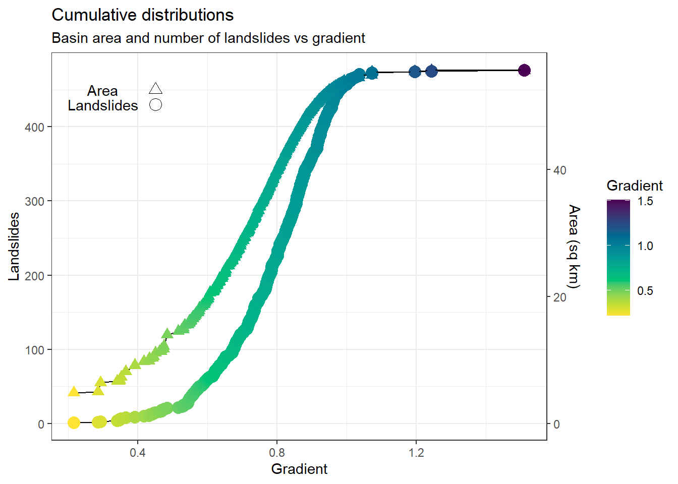
The cumulative area and the cumulative number of landslides can be plotted as a function of a single predictor, as shown below using surface gradient, with gradient here equal to the tangent of the hillslope angle (i.e., rise/run).
Each point plotted along the curve corresponds to one landslide in the inventory. Taking the area and landslide value at each point, another curve showing the cumulative number of landslides versus area can be plotted:
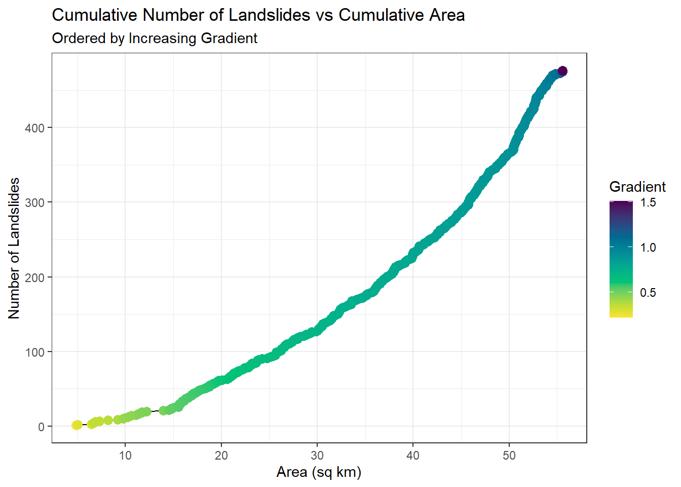
Landslide density is defined as \(\Delta\: landslides/\Delta\: area\), so the slope of this curve gives landslide density. Each location along that curve corresponds to a value of gradient, so these two plots together can be translated to landslide density as a function of gradient.
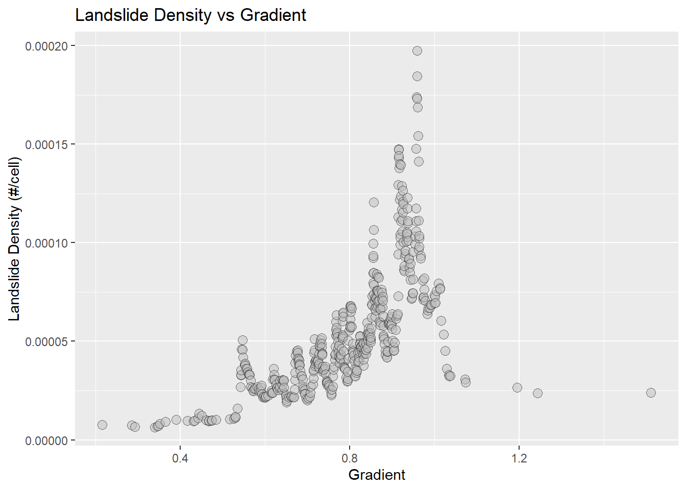
Density in Figure 6 was calculated over a window centered at each landslide point and extending five points up and down the curve. There is considerable scatter in the density values, but also a clear trend indicating very low density at gradients below 55%, increasing density to a peak near 100%, and a very rapid reduction to low values above 100%. Note that density was plotted as number of landslides per DEM cell (this analysis used a 2-meter DEM grid spacing, so four-square-meter cells). This gives the empirical probability of encountering a mapped landslide initiation point in any DEM cell. We want a mathematical expression that will mimic this trend.
We use logistic regression to illustrate this concept. For a set of predictor values \(\textbf{x}\) for some DEM cell, logistic regression expresses the probability that the cell contains a mapped landslide initiation point \(p(\textbf{x})\) as
\[ p( \textbf{x}) = \frac{1}{1+e^{\boldsymbol{-\beta x} } } \]
where \(\boldsymbol{\beta}\) is a vector of empirical coefficients. The ratio of the probability that the cell contains an initiation point and the probability that it does not gives the odds:
\[ \frac{p(\textbf{x})}{1-p(\textbf{x})} = e^{\boldsymbol{\beta x}} = odds \]
The logarithm of the odds is a linear equation in \(\textbf{x}\):
\[ log \left(\frac{p(\textbf{x})}{1-p(\textbf{x})} \right) = \boldsymbol{\beta x} = \beta_0 + \beta_1 x_1 + \beta_2 x_2 + ... + \beta_n x_n = log(odds) \]
For a single predictor, \(log(odds) = \beta_0 + \beta_1 x\). The density shown in Figure 6 gives probability; the logarithm of the odds is shown below:
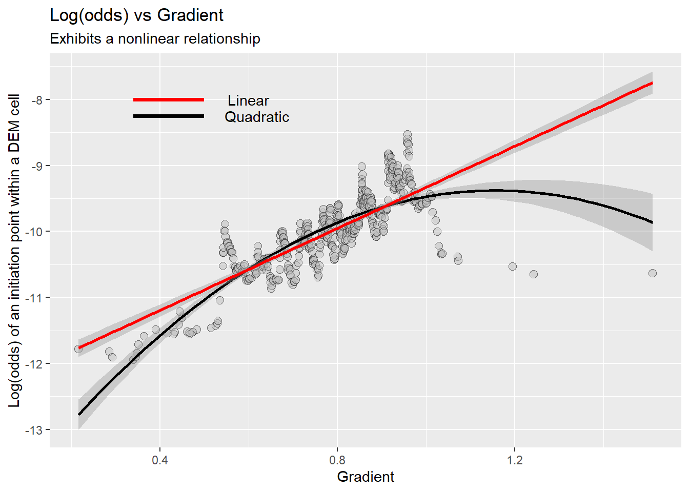
The red line shows a linear fit to these values. In this example, a logistic regression model trained on gradient alone would match observed landslide densities fairly well up to a gradient of 100% and over-predict density at higher gradients. Other types of models might better mimic the observed behavior. For logistic regression, we can remedy this lack-of-fit somewhat by adding an \(x^{2}\) term: \(log(odds) = \beta_0 + \beta_1 x_1 + \beta_2 {x_1}^{2}\), as shown with the black line in Figure 7.
In this dataset, curvature and contributing area exhibited similar patterns:

In the examples above, we looked at how landslide density varies over the range of single predictors. At any predictor value (e.g., at gradient = 0.80), the landslide density indicates the proportion of the area, (i.e., the proportion of DEM cells), with gradients within a small increment of that value that include initiation points. We can look at those proportions directly using density plots. These show the proportion of all initiation points and of all non-initiation-point cells within our sample as a function of predictor value.
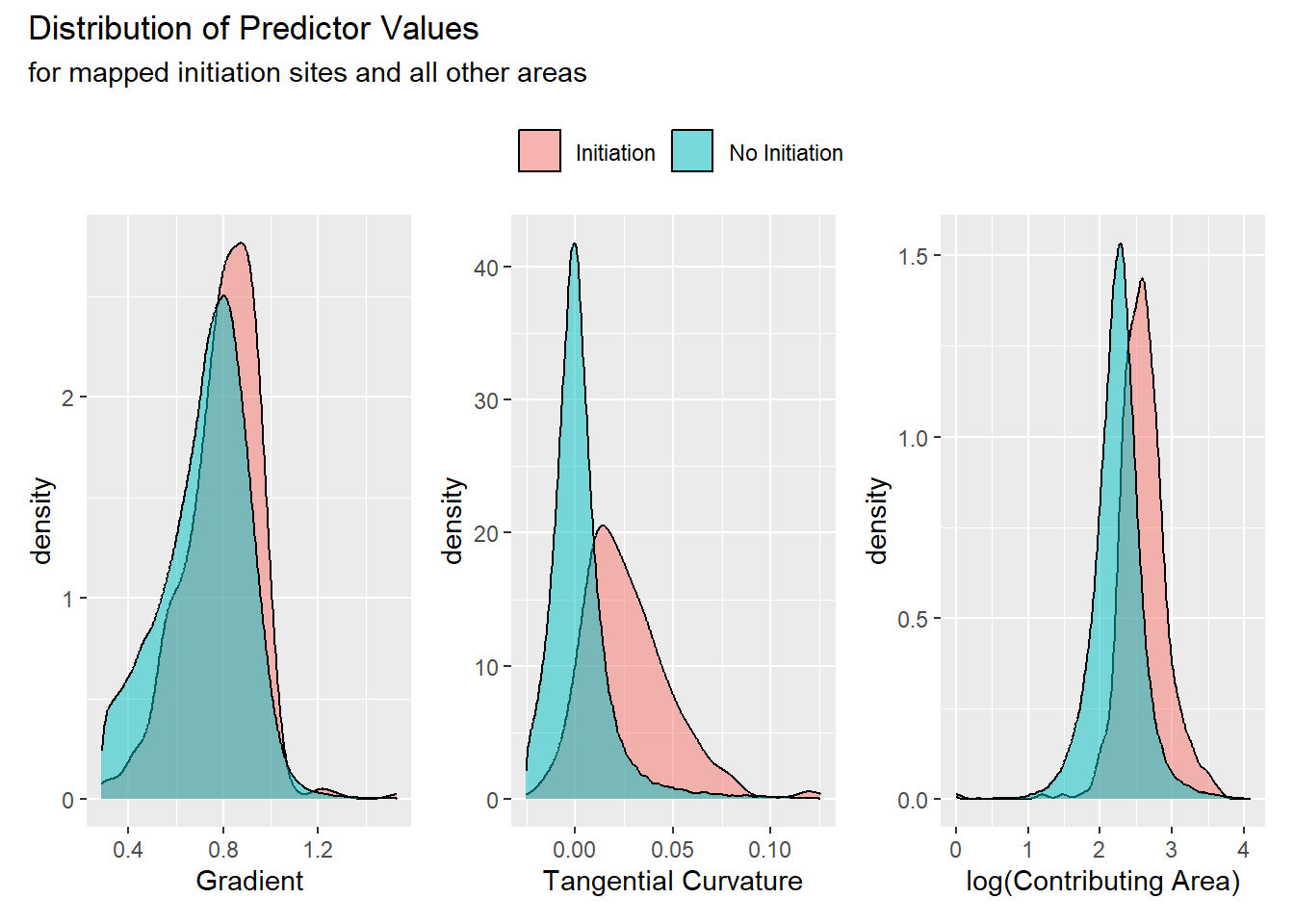
For these examples, the portion of the study area examined was constrained to include only predictor values within the range observed for mapped initiation points. We want to focus on those areas where landslides could occur. Any model should produce a probability of zero for values outside the range of values associated with landslides. We restrict the area examined to that with predictor values within that range to reduce the extent of the data space that must be sampled and characterized. Hence, there is overlap between locations with and without mapped initiation points across the entire range of all predictor values. The degree to which the two distributions differ determine the degree to which conditions associated with initiation sites differ from conditions without initiation sites. For all three of these predictors, initiation sites tend to have slightly larger values than non-initiation sites but, particularly for gradient, the difference is minor. This large degree of overlap can cause gradient to have large standard errors when used in logistic regression, suggesting that gradient has little influence on modeled values. Standard errors with associated z-score and p values are often used as measures of factor importance in model evaluation, but lack of statistical significance in a model is not necessarily indication of lack of causal association [Smith (2018); @chan2022]. We will use machine-learning techniques to examine the influence that different predictors have on model results (Molnar 2023).
So far, we have looked at how landslide density is distributed when all data is projected onto one dimension of the predictor data space. It is challenging to visualize this distribution in a multidimensional data space, but a projection onto two dimensions is informative. Panel A in Figure 10 below shows a heat map of DEM-cell density plotted over gradient and tangential curvature with the landslide point locations overlain. DEM-cell density is calculated as the number of DEM cells counted within within a specified increment of the two variables. Here 500 increments were used in both dimensions, giving 250,000 bins over the range spanned in these plots. The highest landslide-point density is offset from the highest DEM-cell density, so that the highest landslide density, the number of landslide points per unit area shown in Panel B, is offset from both the highest DEM-cell and landslide-point densities. Landslide density here is estimated by summing both the number of landslide points and the number of DEM cells over a specified radius in both dimensions over a regular grid spanning the range of predictor values. I used a grid with 200 increments in each direction and a radius of 20 increments to calculate density. Areas outside the range of observed predictor values are not plotted and areas without any landslide points within that radius are not plotted.
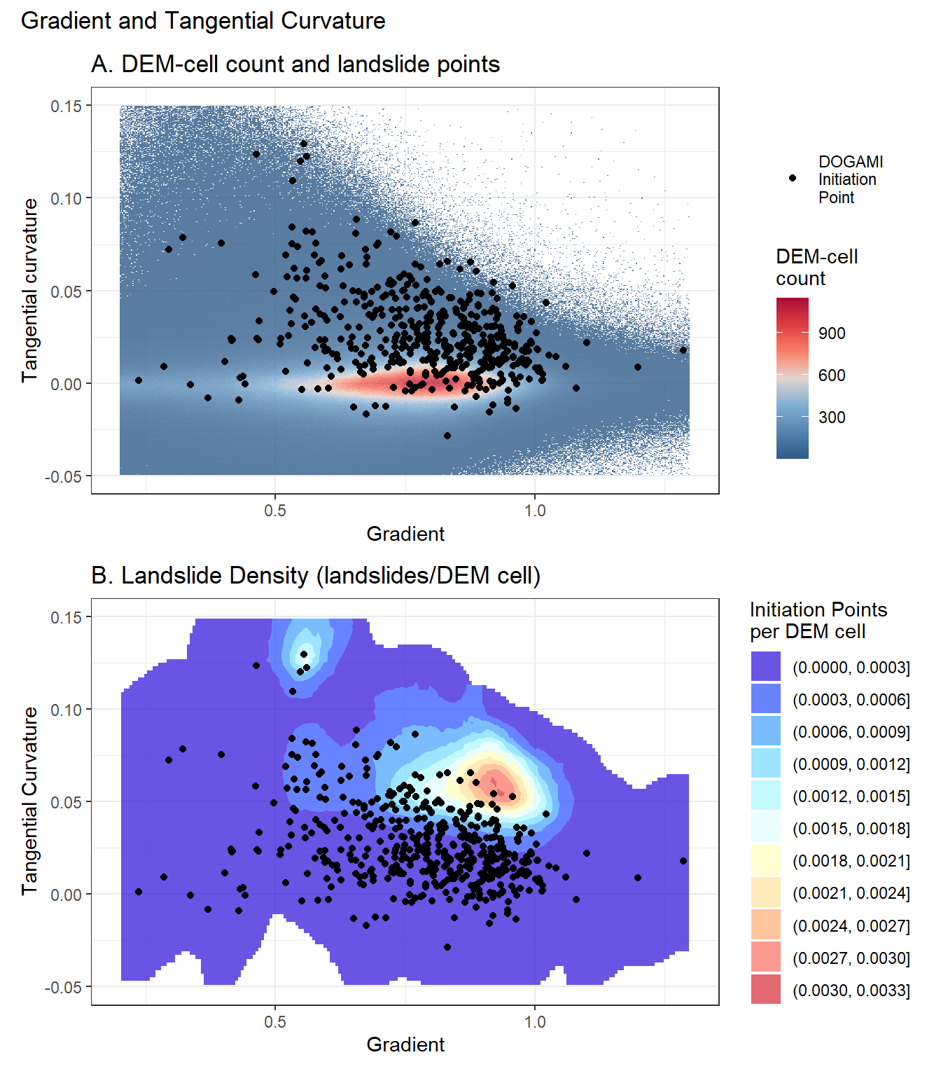
Figure 11 below shows plots of probability calculated with logistic regression. For these calculations, we used all candidate topographic predictors (gradient, tangential curvature, contributing area over 48 hours, total drainage area) for a model with linear terms (Panel A) and another with quadratic terms (Panel B).
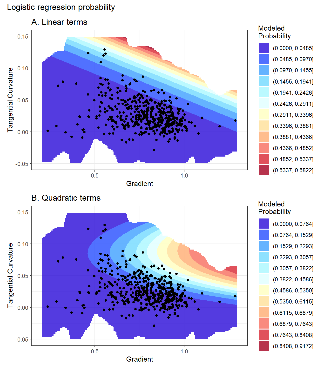
Ideally, the model will produce a pattern of calculated probability similar to that shown in Panel B of Figure 10. Logistic regression uses a linear equation to describe that pattern. In two dimensions, linear terms produce a planar surface and quadratic terms produce a paraboloid surface, neither of which matches the empirical surface particularly well. These plots show a slice through the data space along constant values for all other predictors (tangential curvature = 0.05, drainage area = 20 DEM cells). The absolute values of density and probability differ for two reasons: 1) The empirical density reflects the 13,187,645 cells over the entire DEM within that range of values whereas the modeled probability is only for the 95,200 non-landslide + 476 landslide points used for this example (more on this later) and 2) The linear and quadratic surfaces are fit so that integrating modeled probability across the DEM surface will produce, as closely as possible, the number of observed landslides. The two surfaces are shaped differently, so the magnitude of the fit probabilities at an point in the data space will not match.
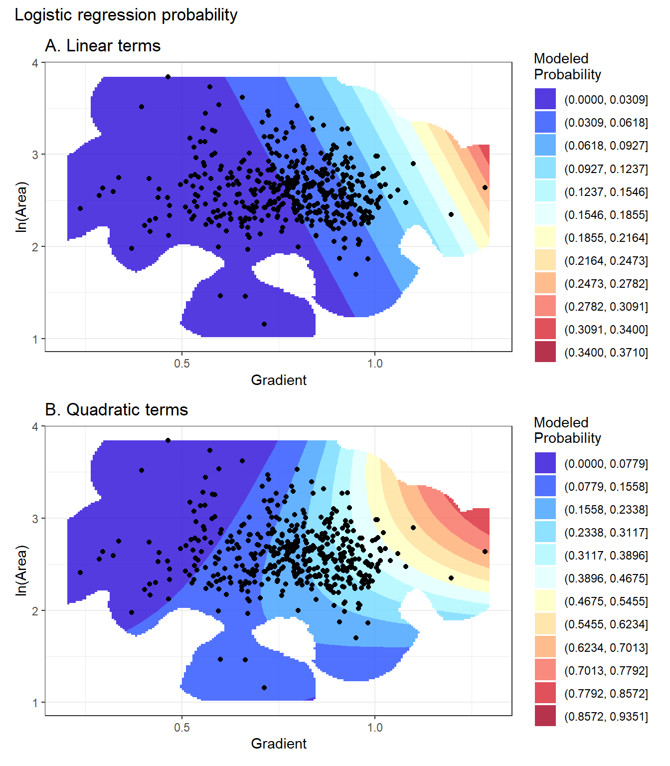
Below are similar figures for gradient and contributing area.

Here are similar plots for log(contributing area) and tangential curvature.


An important feature of these plots to note is the somewhat random locations of the landslide initiation points in those locations where point density is low. When these points fall in regions with low DEM-cell counts, they have a large influence on the empirical landslide density. However, another landslide inventory for the same study sites would have points in slightly different locations in the data space. The empirical pattern of landslide density estimated from a landslide inventory is a noisy approximation of the actual density that would be produced with the complete population of landslide events. A statistical model seeks to match the pattern of density indicated with the inventory data, but the model should not fit that data too tightly, or it will be reproducing noise in the data rather than the underlying pattern of interest.
4.0.1 Model Performance
We need measures of model performance for several tasks.
To compare different algorithms (e.g., logistic regression versus random forest).
To compare models built with different sets of predictors.
To determine how well the model can reproduce what was observed; i.e., how well can it reproduce the spatial distribution of mapped landslide initiation points.
To estimate how well it will predict the spatial distribution of landslide densities when extrapolated to new areas.
To accomplish these tasks, there are five things measures of model performance need to quantify:
How well the sample of nonlandslide points characterizes the joint distributions of predictor values across the entire study area.
How well the chosen model algorithm characterizes the distribution of landslide densities within the data space defined by the predictors.
How well the choice of predictors resolves spatial variations in landslide density.
How sensitive model results are to the predictor values, and
Geomorphic plausability.
Typical measures of model performance include receiver operating characteristic (ROC) curves and the consequent area under the ROC curve (AUC), the precision recall curve (PRC, Yordanov and Brovelli 2020) and the Brier score, among others. All of these are based on some measure of classification success. Given that for our entire sample, we might expect one out of every 30,000 DEM cells to contain a landslide initiation point and there is complete overlap of the distributions of initiation and non-initiation sites within the predictor data space (because we truncated that space to include only values within the range of mapped landslide initiation points), measures based on classification success may be difficult to interpret. Here is an interpretable alternative that can be used for the measures listed above.
The “success-rate” curve was introduced by Chung and Fabbri (2003). To construct a success-rate curve, we rank DEM cells by the modeled probability that they contain a landslide initiation point. We then plot the proportion of mapped landslides versus the proportion of area, ranked by modeled probability. With the calculated probability, we can also plot the proportion of landslides predicted by the model. Classification algorithms preserve the marginal probability of the response (predicted) variable, here landslide density. Integrating density (modeled probability) over area, the same here as summing over DEM cells, gives the number of landslides in the training data. At least it should, if the model is working properly. If the nonlandslide area has been subsampled, which is almost always the case, then the predicted probabilities will be higher than the actual values. This is not a problem, because we plot the proportion of modeled landslides, not the number. Within any increment of modeled probability, integrating the modeled probability values over the area included within those values will give the number, translated to proportion by dividing by the total, of landslides observed within that increment. The curve of proportion of landslides versus proportion of area made by summing ranked probability values over all DEM cells should match exactly the curve for the observed landslides. These curves can be used to examine the first three measures listed above.
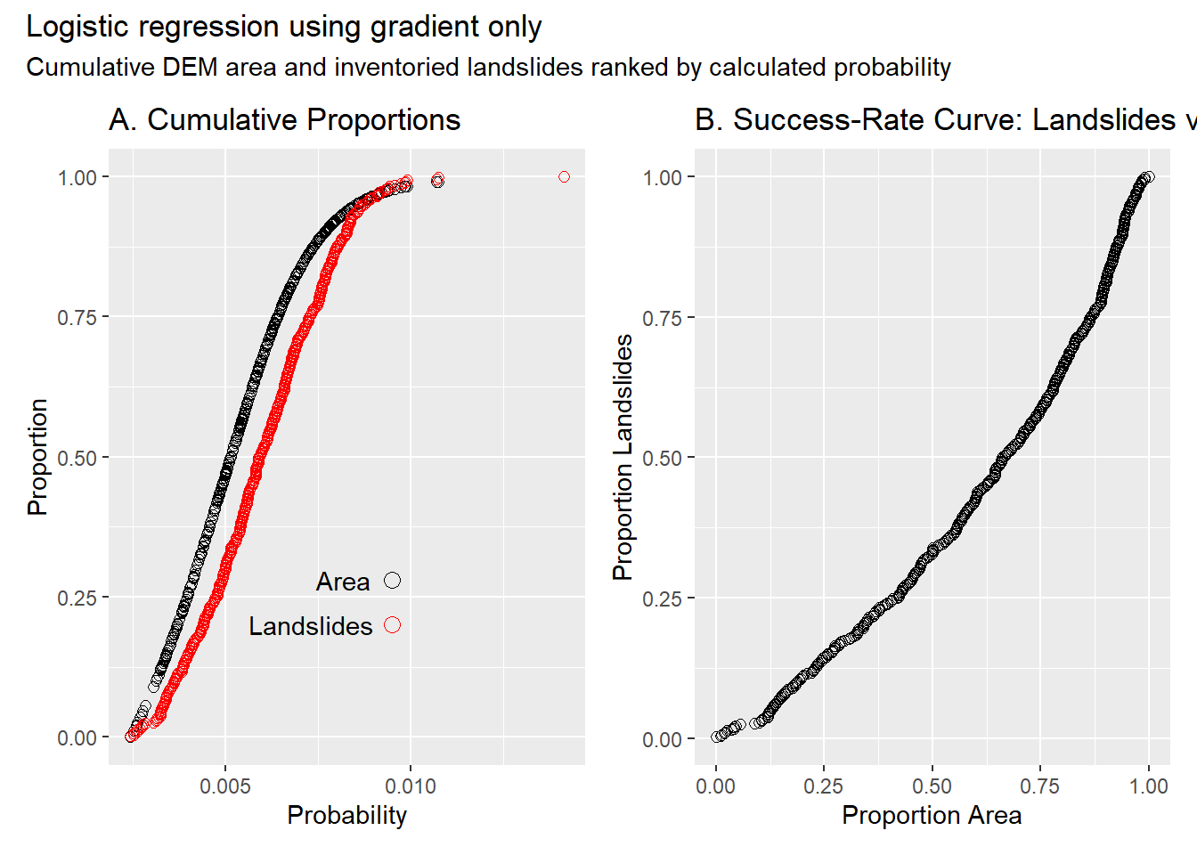
The curves below show results for a logistic regression model using only gradient as a predictor. Each point corresponds to one landslide in the inventory. The cumulative plots in the left panel show how study-site area and mapped landslides are distributed across the range of modeled probability. The success-rate curve in the right panel is built using the proportion of area and proportion of landslide values for each landslide point. If gradient provided no information about the spatial distribution of landslide points, or if the distribution were uniform, the points in the success-rate curve would fall along the diagonal. The degree to which the points curve toward the lower-right corner indicates the degree to which the model resolves spatial variation in landslide density. Smaller area-under-the-curve indicates better resolution.
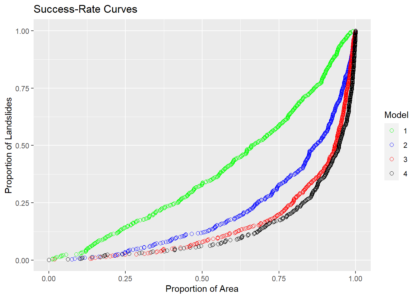
The plot below shows success-rate curves for four logistic regression models:
Gradient only
Gradient + tangential curvature
Gradient + tangential curvature + log(contributing area)
Gradient + gradient2 + curvature + curvature2 + log(CA) + log(CA)2 + log(total contributing area) + log(total contributing area)2 + gradient*curvature + gradient*log(contributing area) + curvature*log(contributing area)
The fourth model includes both total contributing area and quadratic terms. Each additional predictor improves the model’s ability to resolve spatial variability in landslide density, but the amount of increased resolution decreases with each additional predictor. Indeed, although model 4 includes eight more terms than model 3, the success-rate curve indicates little improvement in resolution of spatial variation in landslide density.
At any point along the success-rate curve, the tangent to the curve gives landslide density normalized by the mean density:
\[ \frac{d(Proportion Landslides)}{d(ProportionArea)} = \frac{(\Delta Landslides / Total Landslides)}{(\Delta Area / Total Area)} = \frac{\rho_{Obs}(x)}{\rho bar} \]
Here \(\rho_{Obs}\) indicates the “observed” density indicated by the tangent to the empirical success-rate curve. For a well-performing model, this value will equal the modeled probability. The degree to which the observed density and the modeled probability match provides a measure of how well the set of predictors, the sampled values, and the model algorithm represents actual spatial variability in landslide density. The four plots below compare the modeled probability and the empirical landslide density found from the tangent to the success-rate curve. The tangent was estimated by fitting a quadratic across 11 points. Each plot shows results for a different number of sampled non-landslide points, i.e., different sample balances. The sample balance affects the magnitude of the modeled probability, so the modeled values were normalized by the number of landslides in the inventory divided by the cumulative sum of all modeled DEM-cell probabilities.
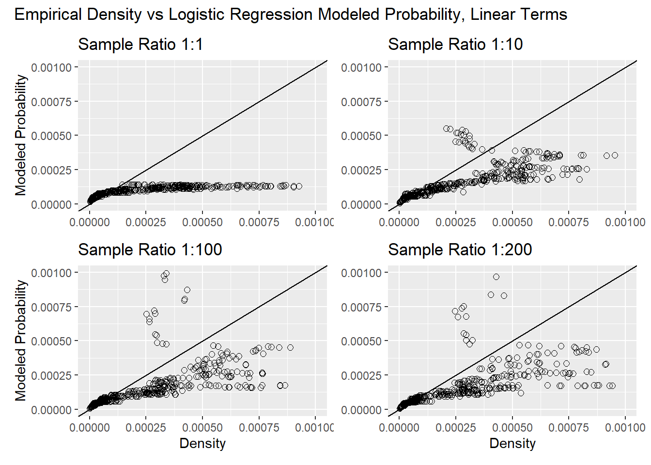
For a well-performing model, the points should plot along a diagonal line with the modeled probability equal to the empirical points. We expect scatter about the diagonal; the inventory provides only a partial sample of the total population of potential landslide locations. For a balanced sample (equal number of landslide and nonlandslide elements in the training sample), the points follow the diagonal only at the very beginning and then the empirical values are much larger than the modeled. The success-rate curve in Figure 17 shows that the area associated with low landslide densities is large compared to the area associated with high landslide densities. The balanced sample has insufficient points in the high-density zones to adequately characterize the distribution of predictor values in those zones. The model was producing probabilities near 1.0 (normalized in the plot above). This is implausible: for even the least stable zones, most sites will not have landslides in the inventory, in part because many will not have sufficient accumulated soil since the last time they failed. A modeled value near 1.0 indicates a lack of nonlandslide sample points in these zones. With larger samples, the points approach, but never quite reach, the diagonal and, at the largest modeled probabilities, the empirical values fall off to lower values. This reflects the inability of the linear terms in this model to match the nonlinear shape of the response term (landslide density) in the data space defined by the predictors, as illustrated Figure 7 and Figure 8. The next set of plots compares the modeled probability and empirical density for model 4 above.
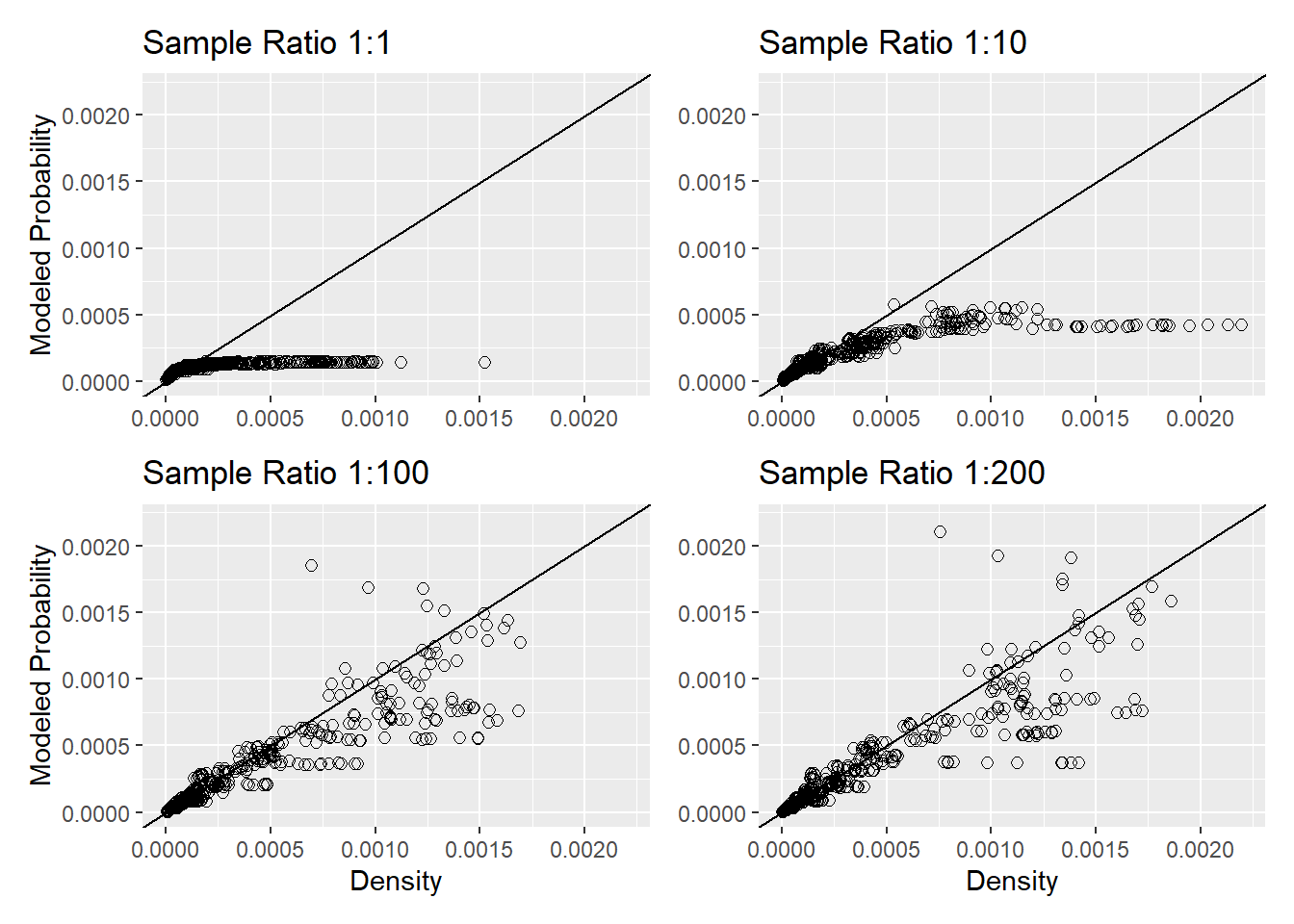
These show a similar pattern with increasing sample size. With small samples, the high-density zones are under sampled. With increasing sample size, the points approach the diagonal across the entire range of modeled probabilities indicating both that the sample size is becoming sufficient to characterize conditions in high-density zones and that the terms in the model can more closely match the shape of the target surface in the multidimensional data space.
This variation in model performance with sample size is seen in comparing success-rate curves built from modeled data (by integrating modeled probability over area) and the observed data from the landslide inventory. Here is an example using the quadratic model described above. The modeled success-rate curves approach closer to the observed curve as the number of nonlandslide points in the sample increases.

The observed success-rate curves in Figure 17 suggest that models 3 and 4 perform about the same, yet Figure 18 and Figure 19 suggest that model 4 better reflects landslide locations in the high-density zones. The high-density zones occupy a relatively small proportion of the study area, so improved resolution there has relatively little influence on the success-rate curve. It is useful to use multiple measures of model performance, since different measures reflect different aspects of how well a model works. As shown with the linear-term model (#3), a numeric measure, such as area under the success-rate curve, may indicate good performance overall yet miss some small but important aspect of model performance. In this case, modeled probabilities for large values of gradient, curvature, and contributing area that were too high.
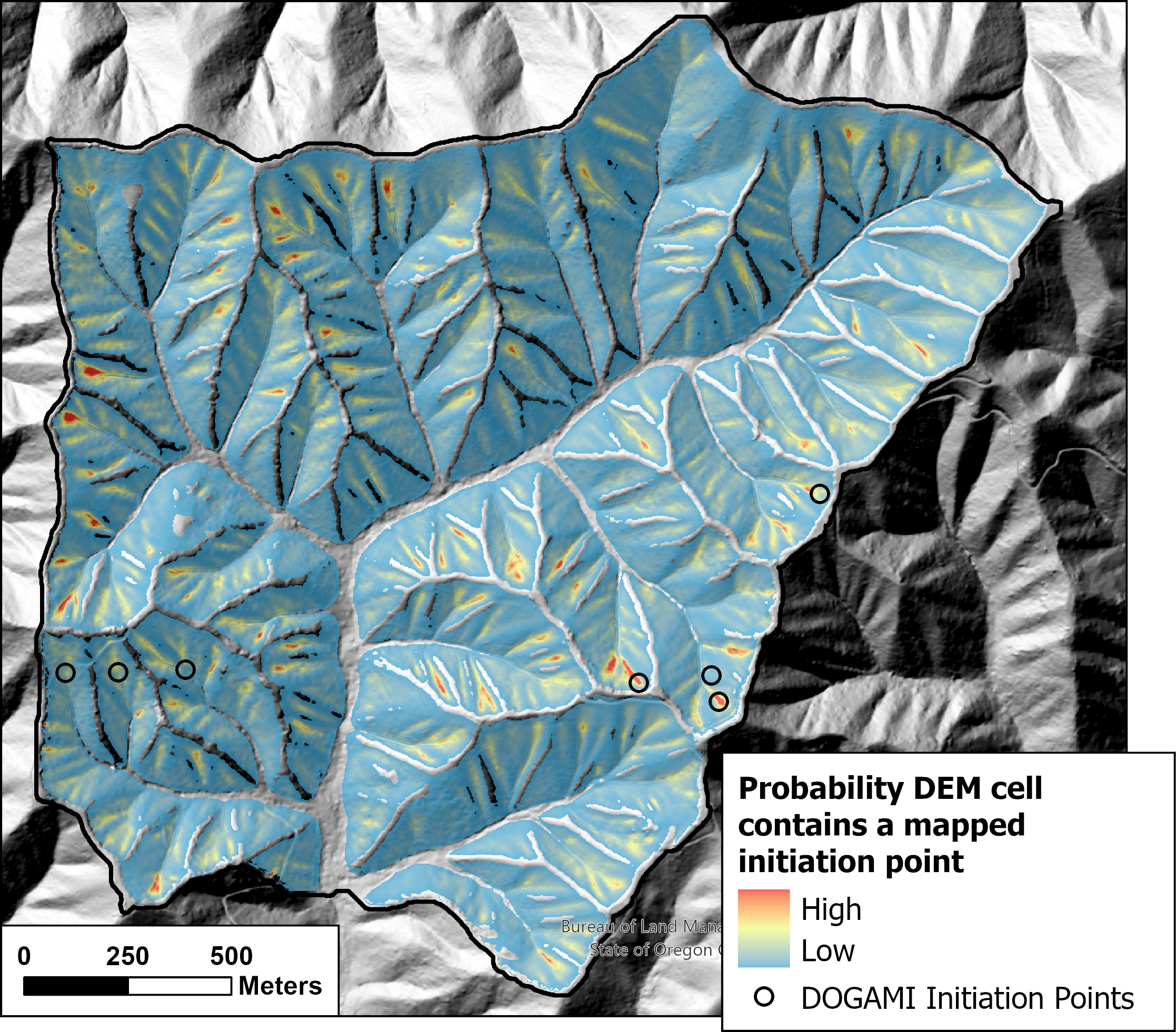
We seek models that can best resolve spatial variability in landslide density. The success-rate curve provides one measure of that ability, but it does not provide a direct prediction by which to gauge model performance when applied to test (rather than training) data. A testable prediction is provided by comparing the proportion of modeled and observed landslides over some specified range of modeled probability. This comparison also provides a measure of model performance. To illustrate, Figure 21 below shows modeled initiation probability for a small basin in the Siuslaw Watershed in Oregon. The model was trained using the DOGAMI Special Paper 53 inventory with a 1:200 ratio of nonlandslide to landslide points.
As discussed above, the integral of modeled probability over space, or summed over DEM cells, gives the modeled number of landslides within those cells. If the sum is over the entire study area, this sum gives the total number of observed landslides. Ordering by modeled probability, summing, and dividing by the total gives a cumulative frequency distribution for the number of landslides ordered by initiation probability, as shown in panel A of Figure 22 below for the linear model with a 1:10 sample ratio.
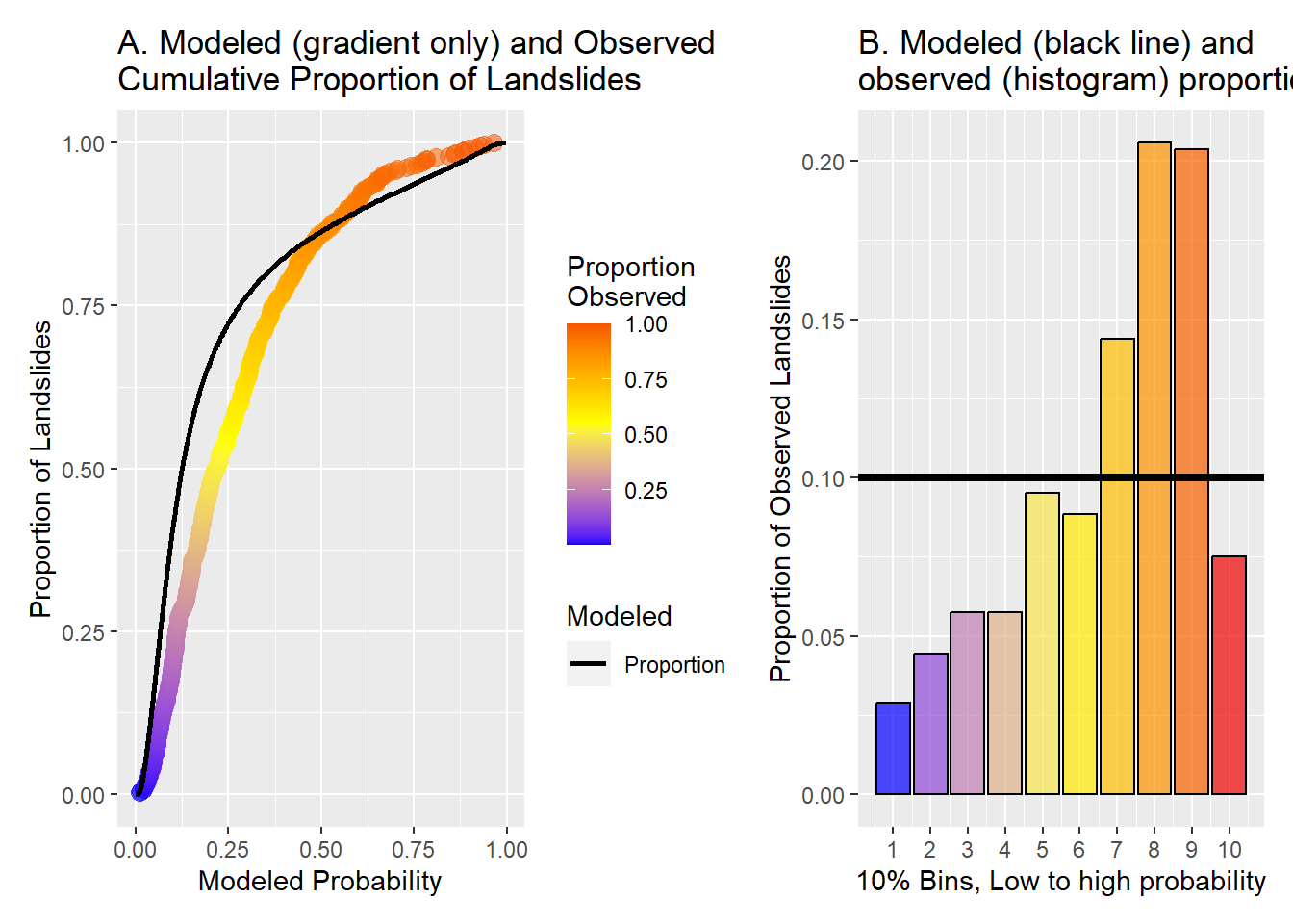
For each DEM cell, there is a one-to-one correspondence between modeled probability and the proportion of modeled and observed landslides. This is translated to a map showing those areas encompassing a given proportion of all landslides as predicted by the model, as shown in Figure 23 below. Over the study area, the area contained within each colored zone is predicted to contain 10% of all observed landslides. (Note that Figure 23 shows only a small portion of the entire study area.)

Over any increment of modeled probability, a good model will predict the same proportion of landslides as observed. Panel B in Figure 22 shows the proportion of observed landslides laying within each 10% increment of modeled landslides over the entire study area used for the DOGAMI inventory. These bins correspond to the 10 rankings in Figure 23. Where the bars fall below 0.1, the model has over-predicted the proportion of landslides; where the bars fall above 0.1, the model has under-predicted the proportion of observed landslides. The sum of the absolute value of these differences provides a measure of model performance based on its ability to match spatial patterns in observed landslide density.
Figure 22 was based on the linear model with a 1:10 ratio of landslide to nonlandslide points in the training data. Figure 24 below shows the misfit, the modeled minus the observed proportion for each modeled 10% bin for the linear and quadratic models with both 1:10 and 1:100 sample ratios.
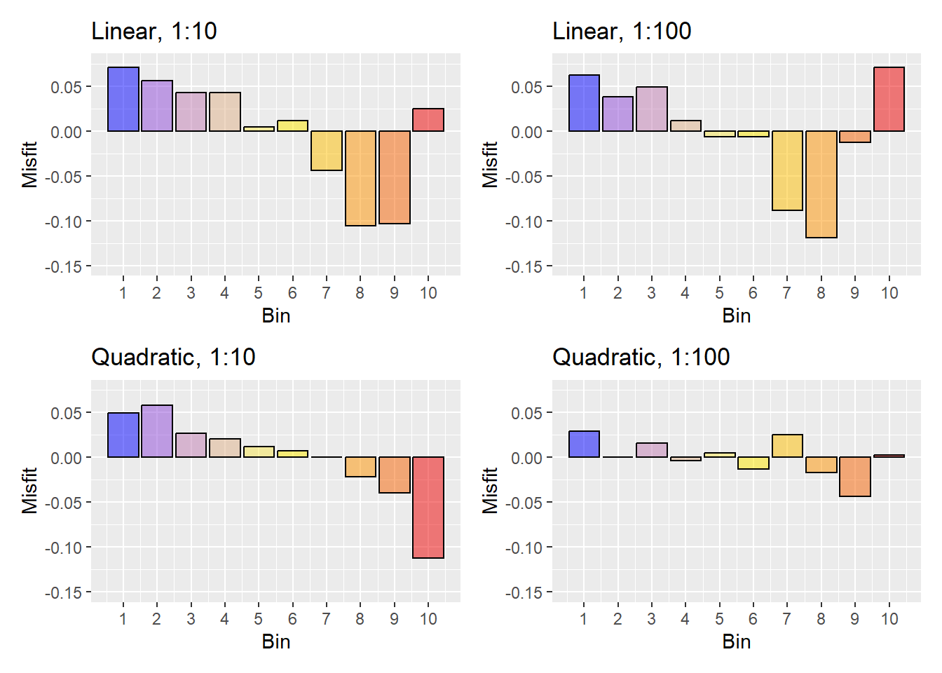
The linear model exhibits systematic differences at both low and high sample ratios. The quadratic model exhibits systematic differences at a low sample ratio, but more random variations at a high sample ratio. These variations may reflect unavoidable noise in the landslide data itself.
The difference sums are listed in Table 1 below:
| Linear | Quadratic | |
|---|---|---|
| 1:10 | 0.506 | 0.347 |
| 1:100 | 0.465 | 0.156 |
Based on ability of each model to replicate observed spatial variations in landslide density, higher sample ratios perform better and the quadratic model performs better than the linear model.
This gives us two measures of model performance: the success-rate curve, which compares the ability of different models to resolve spatial variability in landslide density, and the proportion differences illustrated above, which compare ability of different models to replicate observed spatial variability in landslide density.
We can compare these density-based measures to a measure based on classification success. The ROC curve plots the True Positive Rate versus the False Positive Rate for a range of threshold values spanning the range of modeled probability. The area under the ROC curve (AUC) is used as a single-valued measure of model performance; a higher AUC value indicates a better-performing model. For a given threshold in modeled probability, the True Positive Rate is the number of correctly classified points (True Positives) divided by the total number of landslide points. The False Positive Rate is the number of nonlandslide points incorrectly classified as landslides divided by the total number of nonlandslide points. To build an ROC curve, the TPR and FPR are calculated over the full range of modeled probabilities and the TPR plotted as a function of the FPR. At a very low threshold probability, all points are classified as landslides and both TPR and FPR equal one. At a very high threshold probability, no points are classified as landslides and TPR and FPR are both equal to zero. A model that is good at correctly classifying points in the training sample will have high TPR values and low FPR values, so the plotted curve will approach the upper left corner of the plot. The area under the ROC curve, referred to as AUC, is then a single-valued measure of model performance: higher AUC values indicate a better-performing model.
For a landslide susceptibility model, there are two factors that hinder use of ROC and AUC: 1) most terrain locations where landslides could occur do not have landslides in the inventory but will have a high modeled probability, so the FPR is large no matter how good the model, and 2) ROC should be calculated for the entire DEM, not just the training data, so the FPR becomes a function also of the proportion of DEM area in low and high modeled probability values. Here are ROC curves for the models discussed above:

AUC for each model is listed below.
| Linear | Quadratic | |
|---|---|---|
| 1:10 | 0.867 | 0.883 |
| 1:100 | 0.857 | 0.882 |
The AUC values suggest that the quadratic model is slightly better than the linear model, but also indicates that the 1:10 ratio sample is better than the 1:100-ratio sample for the linear model and that the two sample ratios have almost no effect on model results for the quadratic model. These results are misleading; Table 1 clearly shows that, based on modeled ability to replicate observed spatial patterns in landslide density, the quadratic model is better than the linear model and higher sample ratios are better than lower sample ratios. Other measures of model performance have also been used for evaluating models of susceptibility to landslide initiation, such as the precision-recall curve (Yordanov and Brovelli 2020) and the Brier Score (Woodard et al. 2023). Precision is defined as the number of true positives divided by the sum of true positives and false positives. If the model is accurate, this gives the proportion of potential landslide sites where landslides were observed, which is a function of the sequence of storms over the time period sampled by the landslide inventory. Even a good model will have a precision that is very small because the number of potential landslide sites is far larger than the number of observed landslides. The Brier Score is defined as
\[ B = \frac{1}{N}\sum_{i=1}^N(p_i-o_i)^2 \]
where \(p_i\) is the modeled probability for the \(i^{th}\) DEM cell, \(o_i\) is one if the DEM contains a landslide initiation point and zero otherwise, and the sum is over all \(N\) DEM cells. Smaller Brier Scores indicate better performing models. However, the vast majority of DEM cells have no initiation point, so the Brier Score essentially gives the average squared probability over the DEM, which is not a useful measure of model success. Such measures can be used, but need to be evaluated similarly to how ROC and AUC were examined above.
We have looked so far at model performance in terms of the adequacy of the sample and selected predictors at resolving spatial variability in landslide density using logistic regression. A thorough analysis would apply additional algorithms and use the same measures to compare performance across model types. These could include general additive models, random forest, vector machine, and neural networks, among others. Each model type uses different approaches for characterizing the response (landslide density) surface within the data space defined by the chosen predictors. Some algorithms will work better than others. We have described above some methods by which models can be evaluated, but the actual choice of what predictors to try, what models to use, and how to test them will depend on what is found during the process of data collection and analysis.
Ultimately, however, a model must also be judged by the geomorphic plausibility of the results, which requires making maps and comparing model results to the expectations of people with experience in the area. Discrepancies between model predictions and expectations provide opportunities to re-examine the input data in light of those discrepancies. If the data do not support model results, then the model needs to be modified or the landslide inventory and expert opinions evaluated for errors.
4.0.2 Confidence
So far we have looked at ways to evaluate goodness of fit: how well a model can reproduce the data it was trained with. We want a model that can accurately reproduce observed spatial distributions of landslide density with which to calculate the proportion of landslides expected within different landform types. We also want to know how much confidence to place in the calculated proportions. This is true both for the study area and time period on which the model was trained and also when a model is extrapolated to predict landslide proportions into the future or for locations outside those covered by the landslide inventory. It is not possible to calculate this confidence directly without additional data, but it is possible to estimate it by looking at how sensitive model predictions are to the input data. This sensitivity can be assessed using cross validation, in which a model is trained using a subset of the data and then tested against the remaining data not in that subset. Subsets may be obtained using a random sample from the inventory, or by dividing the study area into different zones, or by subsetting landslides by date of occurrence. This process can be repeated multiple time using different subsets of the inventory with each iteration. The set of model predictions can then be used to calculate confidence intervals for model predictions, in this case, the modeled probability (landslide density) rasters. Each iteration also provides a measure of model performance, such as the difference sums shown in Table 1 above, when a model calibrated to the training subset of the inventory is applied to the remaining test data. The distribution of these performance measures provides an estimate of how poorly the model might perform when applied to new data.
The examples above looked solely at logistic regression. However, each type of model might work well for some cases and not so well for others. It is useful, therefore, to apply more than one model type in an analysis of confidence. I haven’t written code for doing all this yet and so have no examples to show. However, similar ideas are explored by Fabbri and Patera (2021).
References
Amaranthus, M. P., R. M. Rice, N. R. Barr, and R. R. Ziemer. 1985. “Logging and Forest Roads Rleated to Increased Dibris Slides in Southwestern Oregon.” Journal of Forestry 83 (4): 229–33. https://academic.oup.com/jof/article-abstract/83/4/229/4644293.
Benda, L. E., and T. Dunne. 1987. “Sediment Routing by Debris Flow.” In, 213–23. International Association of Hydrological Sciences. Sediment routing by debris flow.
Benda, L. E., D. J. Miller, T. Dunne, G. H. Reeves, and J. K. Agee. 1998. “Dynamic Landscape Systems.” In, 261–88. Springer-Verlag. https://www.researchgate.net/profile/Thomas-Dunne-2/publication/289055083_Dynamic_Landscape_Systems/links/577c051308aece6c20fccf56/Dynamic-Landscape-Systems.pdf.
Benda, Lee. 1990. “The Influence of Debris Flows on Channels and Valley Floors in the Oregon Coast Range, U.S.A.” Earth Surface Processes and Landforms 15 (5): 457–66. https://doi.org/10.1002/esp.3290150508.
Bernard, Thomas G., Dimitri Lague, and Philippe Steer. 2021. “Beyond 2D Landslide Inventories and Their Rollover: Synoptic 3D Inventories and Volume from Repeat Lidar Data.” Earth Surface Dynamics 9 (4): 1013–44. https://doi.org/10.5194/esurf-9-1013-2021.
Bigelow, P. E., L. E. Benda, D. J. Miller, and K. M. Burnett. 2007. “On Debris Flows, River Networs, and the Spatial Structure of Channel Morphology.” Forest Science 53 (2): 220–38. http://www.fs.fed.us/pnw/pubs/journals/pnw_2007_bigelow001.pdf.
Brardinoni, Francesco, Olav Slaymaker, and Marwan A Hassan. 2003. “Landslide Inventory in a Rugged Forested Watershed: A Comparison Between Air-Photo and Field Survey Data.” Geomorphology 54 (3-4): 179–96. https://doi.org/10.1016/s0169-555x(02)00355-0.
Burnett, K. M., and D. J. Miller. 2007. “Streamside Policies for Headwater Channels: An Example Considering Debris Flows in the Oregon Coastal Province.” Forest Science 53 (2): 239–53.
Burns, W. J., J. J. Franczyk, and N. C. Calhoon. 2022. “Protocol for Channelized Debris Flow Susceptibility Mapping.” Special Paper 53. Oregon Department of Geology; Mineral Resources. https://www.oregongeology.org/pubs/sp/SP-53/p-SP-53.htm.
Chung, C., and A. G. Fabbri. 2003. “Validation of Spatial Prediction Models for Landslide Hazard Mapping.” Natural Hazards 30: 451–72. https://www.researchgate.net/profile/Andrea-Fabbri-3/publication/226802573_Validation_of_Spatial_Prediction_Models_for_Landslide_Hazard_Mapping/links/00b49536d1d2219c6b000000/Validation-of-Spatial-Prediction-Models-for-Landslide-Hazard-Mapping.pdf.
Dietrich, W. E., T. Dunne, N. F. Humphrey, and L. M. Reid. 1982. “Construction of Sediment Budgets for Drainage Basins.” In Sediment Budgets and Routing in Forested Drainage Basins, General Technical Report PNW-141, 5–23. US Department of Agriculture, Forest Service.
Dietrich, William E., Dino Bellugi, and Raphael Real de Asua. 2001. “Validation of the Shallow Landslide Model, SHALSTAB, for Forest Management.” In, 195–227. American Geophysical Union. https://doi.org/10.1029/ws002p0195.
Dunne, T. 1991. “Stochastic Aspects of the Relations Between Cliimate, Hydrology and Landform Evolution.” Transactions, Japanese Geomorphological Union 12 (1): 1–24.
Fabbri, Andrea G., and Antonio Patera. 2021. “Spatial Uncertainty of Target Patterns Generated by Different Prediction Models of Landslide Susceptibility.” Applied Sciences 11 (8): 3341. https://doi.org/10.3390/app11083341.
Florinsky, I. V. 2016. Digital Terrain Analysis in Soil Science and Geology. Academic Press, Elsevier.
Gucinski, H., M. J. Furniss, R. R. Ziemer, and M. H. Brookes. 2001. “Forest Roads: A Synthesis of Scientific Information, General Technical Report PNW-GTR-509.” US Department of Agriculture, Forest Service, Pacific Northwest Research Station.
Iida, T. 1999. “A Stochastic Hydro-Geomorphological Model for Shallow Landsliding Due to Rainstorm.” CATENA 34 (3-4): 293–313. https://doi.org/10.1016/s0341-8162(98)00093-9.
Iverson, Richard M. 2014. “Debris Flows: Behaviour and Hazard Assessment.” Geology Today 30 (1): 15–20. https://doi.org/10.1111/gto.12037.
Lima, Pedro, Stefan Steger, Thomas Glade, and Franny G. Murillo-García. 2022. “Literature Review and Bibliometric Analysis on Data-Driven Assessment of Landslide Susceptibility.” Journal of Mountain Science 19 (6): 1670–98. https://doi.org/10.1007/s11629-021-7254-9.
May, Christine L., and Robert E. Gresswell. 2003. “Processes and Rates of Sediment and Wood Accumulation in Headwater Streams of the Oregon Coast Range, USA.” Earth Surface Processes and Landforms 28 (4): 409–24. https://doi.org/10.1002/esp.450.
Miller, Daniel J., and Kelly M. Burnett. 2007. “Effects of Forest Cover, Topography, and Sampling Extent on the Measured Density of Shallow, Translational Landslides.” Water Resources Research 43 (3). https://doi.org/10.1029/2005wr004807.
———. 2008. “A Probabilistic Model of Debris-Flow Delivery to Stream Channels, Demonstrated for the Coast Range of Oregon, USA.” Geomorphology 94 (1-2): 184–205. https://doi.org/10.1016/j.geomorph.2007.05.009.
Molnar, Christoph. 2023. Interpretable Machine Learning, a Guide for Making Black Box Models Explainable. https://christophm.github.io/interpretable-ml-book/.
Montgomery, David R., and William E. Dietrich. 1994. “A Physically Based Model for the Topographic Control on Shallow Landsliding.” Water Resources Research 30 (4): 1153–71. https://doi.org/10.1029/93wr02979.
Montgomery, David R., Kathleen Sullivan, and Harvey M. Greenberg. 1998. “Regional Test of a Model for Shallow Landsliding.” Hydrological Processes 12 (6): 943–55. https://doi.org/10.1002/(sici)1099-1085(199805)12:6<943::aid-hyp664>3.0.co;2-z.
Newman, Daniel R., Jaclyn M. H. Cockburn, Lucian Drǎguţ, and John B. Lindsay. 2022. “Evaluating Scaling Frameworks for Multiscale Geomorphometric Analysis.” Geomatics 2 (1): 36–51. https://doi.org/10.3390/geomatics2010003.
Nowicki Jessee, M. A., M. W. Hamburger, K. Allstadt, D. J. Wald, S. M. Robeson, H. Tanyas, M. Hearne, and E. M. Thompson. 2018. “A Global Empirical Model for Near-Real-Time Assessment of Seismically Induced Landslides.” Journal of Geophysical Research: Earth Surface 123 (8): 1835–59. https://doi.org/10.1029/2017jf004494.
Oregon Department of Forestry. 2022. “Private Forest Accord Report.” Oregon Department of Forestry. https://www.oregon.gov/odf/aboutodf/documents/2022-odf-private-forest-accord-report.pdf.
Patton, Nicholas R., Kathleen A. Lohse, Sarah E. Godsey, Benjamin T. Crosby, and Mark S. Seyfried. 2018. “Predicting Soil Thickness on Soil Mantled Hillslopes.” Nature Communications 9 (1). https://doi.org/10.1038/s41467-018-05743-y.
Penaluna, Brooke E., Gordon H. Reeves, Zanethia C. Barnett, Peter A. Bisson, John M. Buffington, C. Andrew Dolloff, Rebecca L. Flitcroft, et al. 2018. “Using Natural Disturbance and Portfolio Concepts to Guide Aquatic-Riparian Ecosystem Management.” Fisheries 43 (9): 406–22. https://doi.org/10.1002/fsh.10097.
Reid, Leslie M., and Thomas Dunne. 1996. Rapid Evaluation of Sediment Budgets. Reiskirchen, Germany: Catena Verlag.
Rieman, Bruce, Jason Dunham, and James Clayton. 2006. “Emerging Concepts for Management of River Ecosystems and Challenges to Applied Integration of Physical and Biological Sciences in the Pacific Northwest, USA*.” International Journal of River Basin Management 4 (2): 85–97. https://doi.org/10.1080/15715124.2006.9635279.
Riihimäki, H., J. Kemppinen, M. Kopecký, and M. Luoto. 2021. “Topographic Wetness Index as a Proxy for Soil Moisture: The Importance of Flow-Routing Algorithm and Grid Resolution.” Water Resources Research 57 (10). https://doi.org/10.1029/2021wr029871.
Robison, G. E., K. A. Mills, J. Paul, L. Dent, and A. Skaugset. 1999. “Storm Impacts and Landslides of 1996: Final Report.” Oregon Department of Forestry.
Schmidt, K M, J J Roering, J D Stock, W E Dietrich, D R Montgomery, and T Schaub. 2001. “The Variability of Root Cohesion as an Influence on Shallow Landslide Susceptibility in the Oregon Coast Range.” Canadian Geotechnical Journal 38 (5): 995–1024. https://doi.org/10.1139/t01-031.
Shi, X., A. Zhu, J. Burt, W. Choi, R. Wang, T. Pei, B. Li, and C. Qin. 2007. “An Experiment Using a Circular Neighborhood to Calculate Slope Gradient from a DEM.” Photogrammetric Engineering & Remote Sensing 73 (2): 143–54.
Sidle, Roy C. 1991. “A Conceptual Model of Changes in Root Cohesion in Response to Vegetation Management.” Journal of Environmental Quality 20 (1): 43–52. https://doi.org/10.2134/jeq1991.00472425002000010009x.
Skempton, A. W., and F. A. deLory. 1957. “Stability of Natural Slopes in London Clay.” In 4th International Conference on Soil Mechanics and Foundation Engineering, Earth Dams, Slopes and Open Excavations.
Smith, Gary. 2018. “Step Away from Stepwise.” Journal of Big Data 5 (1). https://doi.org/10.1186/s40537-018-0143-6.
Swanson, F. J., R. L. Fredriksen, and F. M. McCorison. 1982. “Material Transfer in a Western Oregon Forested Watershed.” In, 233–66. Hutchinson Ross Publishing Co. https://ir.library.oregonstate.edu/downloads/2b88qd675.
Swanston, D. N., and F. J. Swanson. 1976. “Timber Harvesting, Mass Erosion, and Steepland Forest Geomorphology in the Pacific Northwest.” In Geomorphology and Engineering, 199–221. Dowden, Hutchinson & Ross, Inc.
Tarboton, David G. 1997. “A New Method for the Determination of Flow Directions and Upslope Areas in Grid Digital Elevation Models.” Water Resources Research 33 (2): 309–19. https://doi.org/10.1029/96wr03137.
Turner, Ted R., Steven D. Duke, Brian R. Fransen, Maryanne L. Reiter, Andrew J. Kroll, Jim W. Ward, Janette L. Bach, Tiffany E. Justice, and Robert E. Bilby. 2010. “Landslide Densities Associated with Rainfall, Stand Age, and Topography on Forested Landscapes, Southwestern Washington, USA.” Forest Ecology and Management 259 (12): 2233–47. https://doi.org/10.1016/j.foreco.2010.01.051.
Wilson, J. P., G. Aggett, D. Yongxin, and C. S. Lam. 2008. “Water in the Landscape: A Review of Contemporary Flow Routing Algorithms.” In Advances in Digital Terrain Analysis, 213–36. Springer.
WOLFE, M. D., and J. W. WILLIAMS. 1986. “Rates of Landsliding as Impacted by Timber Management Activities in Northwestern California.” Environmental & Engineering Geoscience xxiii (1): 53–60. https://doi.org/10.2113/gseegeosci.xxiii.1.53.
Woodard, Jacob B., Benjamin B. Mirus, Nathan J. Wood, Kate E. Allstadt, Benjamin A. Leshchinsky, and Matthew M. Crawford. 2023. “Slope Unit Maker (SUMak): An Efficient and Parameter-Free Algorithm for Delineating Slope Units to Improve Landslide Susceptibility Modeling.” http://dx.doi.org/10.5194/nhess-2023-70.
Woodward, Jason S. 2023. “Shallow Landslide Erosion Rates on Industrially Managed Timberlands: Key Factors Affecting Historical and Contemporary Rates.” Environmental & Engineering Geoscience 29 (2): 115–31. https://doi.org/10.2113/eeg-d-22-00005.
Yordanov, V., and M. A. Brovelli. 2020. “Comparing Model Performance Metrics for Landslide Susceptibility Mapping.” International Archives of the Photogrammetry, Remote Sensing and Spatial Information Sciences 43 (3): 1277–84.
Zevenbergen, Lyle W., and Colin R. Thorne. 1987. “Quantitative Analysis of Land Surface Topography.” Earth Surface Processes and Landforms 12 (1): 47–56. https://doi.org/10.1002/esp.3290120107.
Zhu, Jing, Laurie G. Baise, and Eric M. Thompson. 2017. “An Updated Geospatial Liquefaction Model for Global Application.” Bulletin of the Seismological Society of America 107 (3): 1365–85. https://doi.org/10.1785/0120160198.